 Example of a Structural Equation Model
In this example, an employee in a human resources department wants to improve job satisfaction. The example uses the Structural Equation Models platform to analyze responses to a survey of 200 individuals regarding aspects of their job satisfaction. The survey contains responses to 11 questions related to their job satisfaction. You seek to build a structural regression model that relates the answers to the survey questions to the latent variables of leadership characteristics, role conflict, and overall job satisfaction.
1. Select Help > Sample Data Library and open Job Satisfaction.jmp.
2. Select Analyze > Multivariate Methods > Structural Equation Models.
3. Select Support_L through Supervisor_S and click Model Variables.
4. Click OK.
The Structural Equation Models report Model Specification outline appears.
Create Latent Variables
5. Select Support_L through Interact_L in the To List, type Leadership in the box next to Add Latent, and click Add Latent.
6. Select Person_C through Inter_C in the To List, type Conflict in the box next to Add Latent, and click Add Latent.
7. Select General_S through Supervisor_S in the To List, type Satisfaction in the box next to Add Latent, and click Add Latent.
Add Loading and Regression Variables
8. Select Leadership in the From List, select Satisfaction in the To List, and click the unidirectional arrow  button.
9. Select Leadership in the From List, select Conflict in the To List, and click the unidirectional arrow button.
10. Select Conflict in the From List, select Satisfaction in the To List, and click the unidirectional arrow button.
11. In the text box below Model Name (in the top left of the Model Specification report), type Path Analysis with Latent Variables.
12. Click Run.
13. (Optional.) Click the red triangle next to Structural Equation Model: Path Analysis with Latent Variables and select Path Diagram > Layout > 6.
14. (Optional.) Click the gray disclosure icon next to Parameter Estimates.
Closing the Parameter Estimates report enables you to see the entire path diagram.
Figure 8.2 Structural Equation Model Report
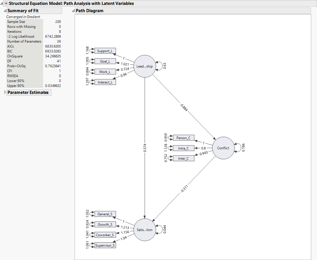
The chi-square statistic for this model, listed in the Summary of Fit report, is 34.27 with 41 degrees of freedom. Note that the corresponding p-value is 0.7624, which is not significant. This indicates that there is not evidence to reject the null hypothesis that the model fits well. Therefore, you conclude that this model fits the data reasonably well.
The chi-square value depends on the sample size, and thus, some well-fitting models can still produce a significant chi-square value. The comparative fit index (CFI) and root mean square error of approximation (RMSEA) provide additional guidance for determining model fit. These indices are bounded between 0 and 1. CFI values greater than 0.90 and RMSEA values less than 0.10 are preferred (Browne and Cudeck 1993; Hu and Bentler 1999). Here, the CFI of 1 and RMSEA of 0 indicate an excellent fit.
15. Click the red triangle next to Structural Equation Model: Path Analysis with Latent Variables and select Standardized Parameter Estimates.
Figure 8.3 Standardized Parameter Estimates Report
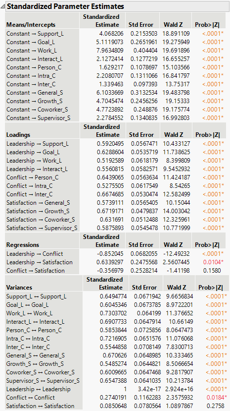
The estimates for the Loadings in the Standardized Parameter Estimates report help explain the measurement model that defines the latent variables. Standardized loadings are the correlation of the observed variable with the unobserved latent variable. Loadings for all latent variables in the report range from 0.52 to 0.67, which suggests well-defined constructs for Leadership, Conflict, and Satisfaction.
In Figure 8.2, the parameter estimates under Regressions suggest a negative effect of Leadership on Conflict and of Conflict on Satisfaction, whereas Leadership has a positive effect on Satisfaction. Thus, higher scores on Leadership are associated with lower Conflict and more Satisfaction, and higher scores in Conflict are associated with lower scores in Satisfaction. The corresponding p-values for the parameter estimates are shown under Regressions. The Leadership -> Conflict and Leadership -> Satisfaction regression parameters are both significant at the α = 0.05 level. Therefore, you conclude that those regression relationships are strong.
Note: You can also use the Regression parameter estimates in the Standardized Parameter Estimates report as effect sizes. These effect sizes are interpreted as the change in standard deviation units in the outcome for a one standard deviation change in the predictor.
16. Click the red triangle next to Structural Equation Model: Path Analysis with Latent Variables and select Normalized Residuals Heat Map.
Figure 8.4 Normalized Residuals Heat Map
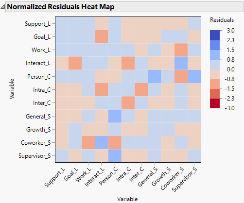
The Normalized Residuals Heat Map has no values that exceed 2.0 units in the positive or negative direction; this is further evidence that the model fits the data well. The residuals can also diagnose ill-fitting models at a more granular level. The normalized residuals in this model do not show evidence of local misfit.