Example of Partial Least Squares
This example is from spectrometric calibration, which is an area where partial least squares is very effective. Suppose you are researching pollution in the Baltic Sea. You would like to use the spectra of samples of sea water to determine the amounts of three compounds that are present in these samples.
The three compounds of interest are:
• lignin sulfonate (ls), which is pulp industry pollution
• humic acid (ha), which is a natural forest product
• an optical whitener from detergent (dt)
The amounts of these compounds in each of the samples are the responses. The predictors are spectral emission intensities measured at a range of wavelengths (v1–v27).
For the purposes of calibrating the model, samples with known compositions are used. The calibration data consist of 16 samples of known concentrations of lignin sulfonate, humic acid, and detergent. Emission intensities are recorded at 27 equidistant wavelengths. Use the Partial Least Squares platform to build a model for predicting the amount of the compounds from the spectral emission intensities.
1. Select Help > Sample Data Library and open Baltic.jmp.
Note: The data in the Baltic.jmp data table are reported in Umetrics (1995). The original source is Lindberg, Persson, and Wold (1983).
2. Select Analyze > Multivariate Methods > Partial Least Squares.
3. Assign ls, ha, and dt to the Y, Response role.
4. Assign Intensities, which contains the 27 intensity variables v1 through v27, to the X, Factor role.
5. Click OK.
The Partial Least Squares Model Launch control panel appears.
6. Select Leave-One-Out as the Validation Method.
7. Click Go.
Since the van der Voet test is a randomization test, your Prob > van der Voet T2 values may differ slightly.
Figure 6.2 Partial Least Squares Report
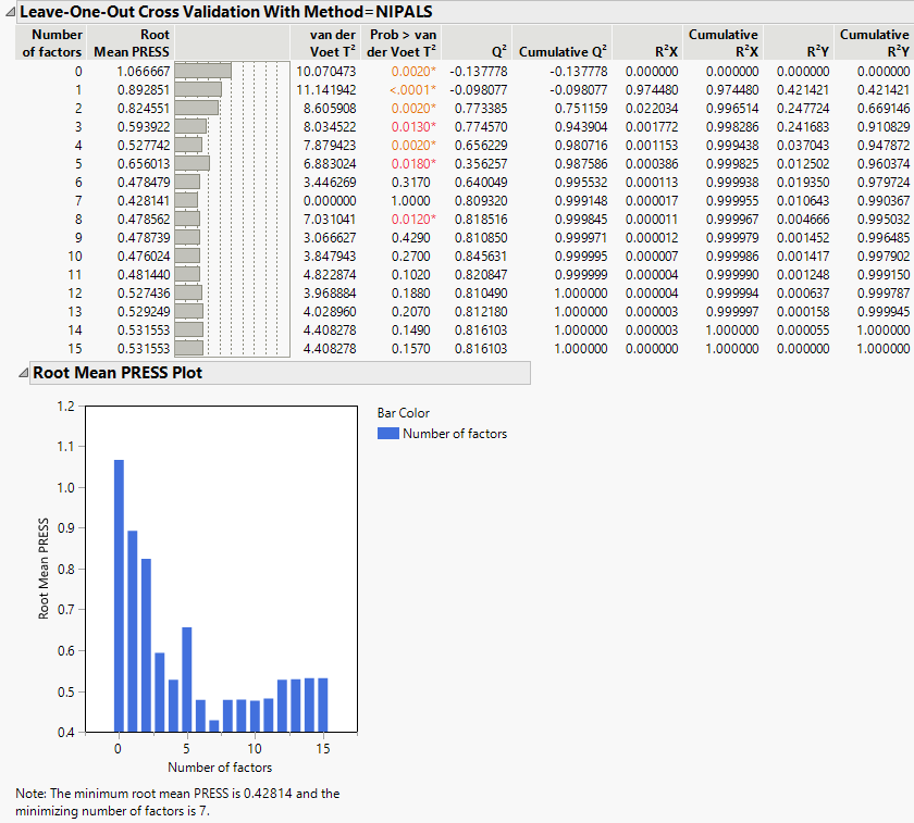
The Root Mean PRESS (predicted residual sum of squares) Plot shows that Root Mean PRESS is minimized when the number of factors is 7. This is stated in the note beneath the Root Mean PRESS Plot. A report called NIPALS Fit with 7 Factors is produced. A portion of that report is shown in Figure 6.3.
The van der Voet T2 statistic tests to determine whether a model with a different number of factors differs significantly from the model with the minimum PRESS value. A common practice is to extract the smallest number of factors for which the van der Voet significance level exceeds 0.10 (SAS Institute Inc 2018f; Tobias 1995). If you were to apply this thinking here, you would fit a new model by entering 6 as the Number of Factors in the Model Launch panel.
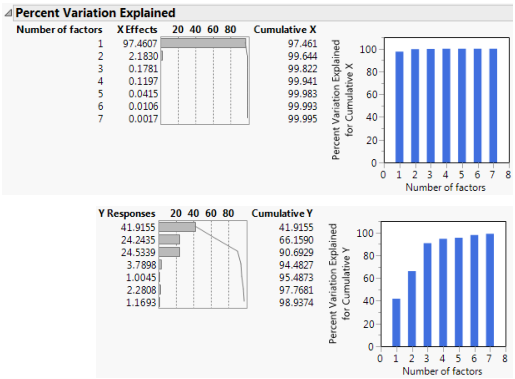
Figure 6.3 Seven Extracted Factors
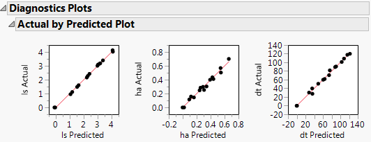
8. Click the NIPALS Fit with 7 Factors red triangle and select Diagnostics Plots.
This gives a report showing actual by predicted plots and three reports showing various residual plots. The Actual by Predicted Plot shows the degree to which predicted compound amounts agree with actual amounts.
Figure 6.4 Diagnostics Plots
9. Click the NIPALS Fit with 7 Factors red triangle and select VIP vs Coefficients Plot.
Figure 6.5 VIP vs Coefficients Plot
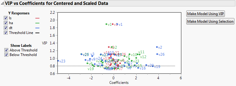
The VIP vs Coefficients plot helps identify variables that are influential relative to the fit for the various responses. For example, v23, v2, and v26 have both VIP values that exceed 0.8 and relatively large coefficients.