Handle()
Handle() places a marker at the coordinates given by the initial values of the first two arguments and draws the graph using the initial values of the arguments. You can then click and drag the marker to move the handle to a new location. The first script is executed at each mousedown to update the graph dynamically, according to the new coordinates of the handle. The second script (optional, and not used here) is executed at each mouseup, similarly; see the example for Mousetrap().
// Normal Density
mu = 0;
sigma = 1;
rsqrt2pi = 1 / Sqrt( 2 * Pi() );
win = New Window( "Normal Density",
Graph Box(
Frame Size( 500, 300 ),
X Scale( -3, 3 ),
Y Scale( 0, 1 ),
Y Function( Normal Density( (x - mu) / sigma ) / sigma, x );
Handle(
mu,
rsqrt2pi / sigma,
mu = x;
sigma = rsqrt2pi / y;
);
Text( {1, .7}, "mu ", mu, {1, .65}, "sigma ", sigma );
)
);
Run demoPlotProb.jsl in the JMP Samples/Scripts folder to see Beta Density, Gamma Density, Weibull Density, and LogNormal Density graphs. The output for Normal Density is shown in Figure 12.23. Because we cannot show you the picture in motion, be sure to run this script yourself.
Figure 12.23 Normal Density Example for Handle()
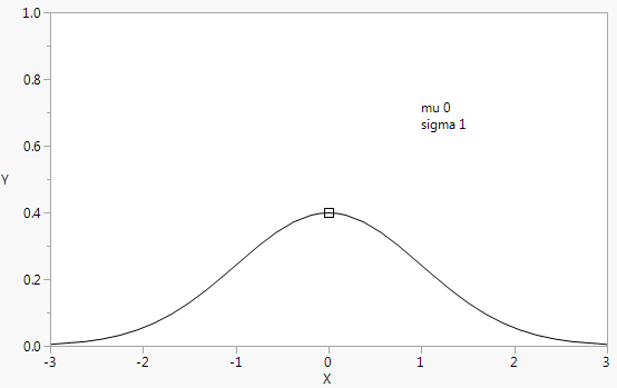
To avoid errors, be sure to set the initial values of the handle’s coordinates, as in the first line of this example.
If you want to use some function of a handle’s coordinates, such as in the normal density example, you should adjust the arguments for Handle(). Otherwise, the handle marker would run away from the mouse.
Y Function( a * x ^ b );
Handle( a, b, a = 2 * x, b = y );
Suppose you drag the marker from its initial location to (3,4). The argument a is set to 6 and b to 4; the graph is redrawn as Y = 6x4; and the handle is now drawn at (6,4), several units away from the mouse. To compensate, you would adjust the first argument to handle, for example.
Handle( a / 2, b, a = 2 * x; b=y );
To generalize, suppose you define the Handle() arguments as functions of the handle’s (x, y) coordinates. For example, a=f(x) and b=g(y). If f(x)=x and g(y)=y, then you would specify simply a,b as the first two arguments. If not, you would solve a = f(x) for x and solve b = g(y) for y to get the appropriate arguments.
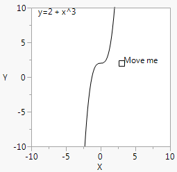
You can use other functions to constrain Handle(). For example, here is an interactive graph to demonstrate power functions that uses Round() to prevent bad exponents and to keep the intercepts simple.
a = 3;b = 2;win = New Window( "Intercepts and Powers",
Graph Box(Frame Size( 200, 200 ),
X Scale( -10, 10 ),
Y Scale( -10, 10 ),
Y Function( Round( b ) + x ^ (Round( a )), x );
Handle(a,
b,
a = x;
b = y;
);
Text( {a, b}, " Move me" );
Text( {-9, 9}, "y=", Round( b ), " + x^", Round( a ) );
)
);
Figure 12.24 Intercepts and Powers for Handle()
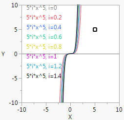
Handle() and For() can be nested for complex graphs.
a = 5;b = 5;win = New Window( "Powers",
Graph Box(Frame Size( 200, 200 ),
X Scale( -10, 10 ),
Y Scale( -10, 10 ),
For( i = 0, i < 1.5, i += .2,
Pen Color( 1 + 10 * i );
Text Color( 1 + 10 * i );
Y Function( i * x ^ Round( a ), x );
Handle(a,
b,
a = x;
b = y;
);
h = 9 - 10 * i;
Text( {-9, h}, b, "*i*x^", Round( a ), ", i=", i );
) ) );
Figure 12.25 Nested Handle() and For()
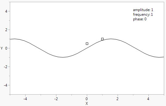
You can use more than one handle in a graph:
amplitude = 1;freq = 1;phase = 0;win = New Window( "Sine Wave",
Graph Box(Frame Size( 500, 300 ),
X Scale( -5, 5 ),
Y Scale( -5, 5 ),
Y Function( amplitude * Sine( x / freq + phase ), x );
Handle( // first handle
freq,
amplitude,
freq = x;
amplitude = y;
);
Handle( phase, .5, phase = x ); // second handle
Text( {3, 4}, "amplitude: ",Round( amplitude, 4 ),
{3, 3.5}, "frequency: ",Round( freq, 4 ),
{3, 3}, "phase: ",Round( phase, 4 )
);
)
);
Figure 12.26 Two Handles