Model Outlines
The outline for each model contains a red triangle menu with the following option:
Remove
Removes the model outline from the report and removes the model from the Model List.
The outline for each model contains the following reports:
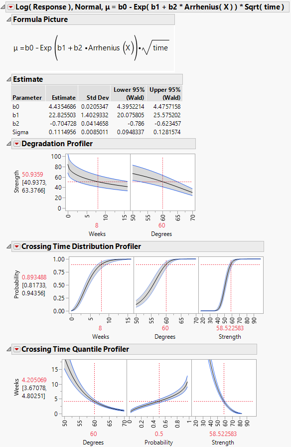
Formula Picture
Shows the equation for the location parameter.
Estimate
Shows parameter estimates and their standard deviations. This report also contains 95% Wald-based confidence intervals for the parameters.
Note: If you specify a reference temperature (X0), this value is also displayed at the top of the Estimate report.
Distribution, Quantile, and Inverse Prediction
For more information about the profilers, see Profilers.
Residual Plots
For more information about the residual plots, see Residual Plots.
Figure 8.15 Reports within a Model Outline
Profilers
Three profilers appear in the model report.
Degradation Profiler
The Degradation Profiler shows a profiler view of the Degradation Data Analysis plot for the given model. The response is the degradation response Y. The profiler includes a plot against the Time variable and a plot against the optional explanatory variable X (if you have specified one). The plot against Time shows the median of the fitted distribution of Y as a solid curve. The dashed curves show the 0.025 and 0.975 percentiles of the fitted distribution of Y.
Crossing Time Distribution Profiler
Use the Crossing Time Distribution Profiler to determine the probability that the degradation measurement falls below a given threshold at some point in time.
The profiler plots the estimated cumulative distribution function of the response Y as a function of Time, the optional X variable, and Y. The plots for Time and Y show Wald confidence intervals.
Crossing Time Quantile Profiler
Use the Crossing Time Quantile Profiler to determine the time at which a specified proportion of measurements falls below a given threshold value.
The profiler plots the estimated Time as a function of the optional X variable, quantile values for Y (Probability), and Y. The plots for Probability and Y show Wald confidence intervals.
Residual Plots
Four residual plots appear in the model report. Use these plots to validate the distributional assumption for the model. For more information about the standardized residuals, see Statistical Details for the Destructive Degradation Platform.
Cox-Snell Residual P-P Plot
If the points deviate far from the diagonal, then the distributional assumption might be violated. The Cox-Snell Residual P-P Plot red triangle menu has an option called Save Residuals that enables you to save the residual data to the data table. See Meeker and Escobar (1998, sec. 17.6.1) for a discussion of Cox-Snell residuals.
Probability Plot of Standardized Residuals
If the points deviate far from the diagonal, then the distributional assumption might be violated. The Probability Plot of Standardized Residuals red triangle menu has an option called Save Residuals that enables you to save the residual data to the data table.
Standardized Residuals versus Time
Use the Standardized Residuals versus Time plot to examine differences in variability over time. The Standardized Residuals versus Time red triangle menu has an option called Save Residuals that enables you to save the residual data to the data table.
Standardized Residuals versus Predicted
Use the Standardized Residuals versus Predicted plot to examine differences in variability over the range of predicted values. The Standardized Residuals versus Predicted red triangle menu has an option called Save Residuals that enables you to save the residual data to the data table.