Model Report
The time series modeling options are used to fit theoretical models to the series and use the fitted model to predict (forecast) future values of the series. These options also produce statistics and residuals that enable you to determine the adequacy of the model that you have chosen to use. You can select the modeling options multiple times. Each time you select a model, that model is added to the Model Comparison table. a report of the results of the fit and a forecast is added to the Time Series report window. When the Report check box next to a model in the Model Comparison table is selected, a report is produced for that model. The report specifies the model in its title.
The following reports are shown by default:
• Model Summary Table
• Parameter Estimates Table
• Forecast Plot
• Residuals
• Iteration History
Model Summary Table
The Model Summary table contains fit statistics for the model. In the formulas below, n is the length of the series and k is the number of fitted parameters in the model.
DF
The number of degrees of freedom in the fit, n – k.
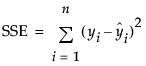
Sum of Squared Errors
The sum of the squared residuals.
Variance Estimate
The unconditional sum of squares (SSE) divided by the number of degrees of freedom (n – k). The variance estimate is computed as SSE / (n – k). This is the sample estimate of the variance of the random shocks at, described in the section ARIMA Model.
Standard Deviation
The square root of the variance estimate. This is a sample estimate of the standard deviation of the random shocks at.
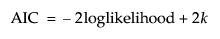
Akaike’s Information Criterion [AIC]
Smaller AIC values indicate better fit. AIC is computed as follows:
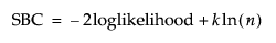
Schwarz’s Bayesian Criterion [SBC or BIC]
Smaller SBC values indicate better fit. Schwarz’s Bayesian Criterion is equivalent to the Bayesian Information Criterion (BIC). SBC is computed as follows:
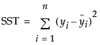
RSquare
The R-Square is computed as follows:

where
 are the one-step-ahead forecasts
 is the mean yi
If the model does not fit the series well, the model error sum of squares, SSE, might be larger than the total sum of squares, SST. As a result, R2 can be negative.
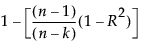
RSquare Adj
The adjusted R2 is computed as follows:
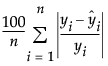
MAPE
The Mean Absolute Percentage Error is computed as follows:
MAE
The Mean Absolute Error is computed as follows:

–2LogLikelihood
Twice the negative log-likelihood function evaluated at the best-fit parameter estimates. Smaller values are better fits. See Likelihood, AICc, and BIC in Fitting Linear Models.
Stable
Indicates whether the autoregressive operator is stable. That is, whether all the roots of φ(z) = 0 lie outside the unit circle.
Invertible
Indicates whether the moving average operator is invertible. That is, whether all the roots of θ(z) = 0 lie outside the unit circle.
Note: The φ and θ operators are defined in the section ARIMA Model.
Parameter Estimates Table
There is a Parameter Estimates table for each selected fit, which gives the estimates for the time series model parameters. Each type of model has its own set of parameters, which are described in the sections on specific time series models. Each Parameter Estimates table contains the following columns:
Term
The name of the parameter, which are described in the sections for each model type. Some models contain an intercept or mean term. In those models, the related constant estimate is also shown. The definition of the constant estimate is given under the description of ARIMA models.
Factor
(Shown only for multiplicative Seasonal ARIMA models.) The factor of the model that contains the parameter. In the multiplicative seasonal models, Factor 1 is nonseasonal and Factor 2 is seasonal.
Lag
(Shown only for ARIMA and Seasonal ARIMA models.) The degree of the lag or backshift operator that is applied to the term to which the parameter is multiplied.
Estimate
The parameter estimates of the time series model.
Std Error
The estimates of the standard errors of the parameter estimates. These estimates are used to calculate tests and prediction intervals.
t Ratio
The test statistics for the hypotheses that each parameter is zero. The test statistic for a parameter is the ratio of the parameter estimate to its standard error. If the hypothesis is true, then this statistic has an approximate Student’s t distribution. Looking for a t-ratio greater than 2 in absolute value is a common rule for judging significance because it approximates the 0.05 significance level.
Prob>|t|
The observed p-value calculated for each parameter. The p-value is the probability of getting a t-ratio greater (in absolute value) than the computed value, given a true hypothesis.
Constant Estimate
Shown for models that contain an intercept or mean term. The definition of the constant estimate is given under ARIMA model.
Mu
(Shown only for ARIMA and Seasonal ARIMA models.) The estimate for the intercept value of an ARIMA or seasonal ARIMA model.
Forecast Plot
Each model has its own Forecast plot. The Forecast plot shows both the observed and predicted values for the time series. The plot is divided by a vertical line into two regions. To the left of the vertical line, the one-step-ahead forecasts are overlaid with the observed data points. To the right of the vertical line are the future values forecast by the model and the prediction intervals for the forecast.
You can control the number of future forecast values by changing the setting of the Forecast Periods option in the platform launch window or by selecting Number of Forecast Periods from the Time Series red triangle menu.
Residuals
The graphs in the Residuals report show the values of the residuals based on the fitted model. These values are the observed values of the time series minus the one-step-ahead predicted values. The autocorrelation and partial autocorrelation reports for these residuals are also shown. These reports can be used to determine whether the fitted model is adequate to describe the data. If the fitted model is adequate, the points in the residual plot should be normally distributed about zero and the autocorrelation and partial autocorrelation of the residuals should not have any significant components for lags greater than zero.
Iteration History
The model parameter estimation is an iterative procedure by which the log-likelihood is maximized by adjusting the estimates of the parameters. The Iteration History report is shown for each model, and it contains the value of the objective function at each iteration. This can be useful for diagnosing problems with the fitting procedure. Attempting to fit a model that is poorly suited to the data can result in a failure to converge on an optimum value for the likelihood. The Iteration History table contains the following quantities:
Iter
The iteration number.
Iteration History
The objective function value for each step.
Step
The type of iteration step.
Obj-Criterion
The norm of the gradient of the objective function.
Model Report Options
Each model report has a red triangle menu that contains the following options:
Show Points
Shows or hides the data points in the forecast graph.
Show Prediction Interval
Shows or hides the prediction intervals in the forecast graph.
Save Columns
Creates a new data table that contains columns that represent the results of the model.
Save Prediction Formula
Saves the data and prediction formula to a new data table.
Create SAS Job
Creates SAS code that duplicates the model analysis in SAS.
Submit to SAS
Submits SAS code to SAS that duplicates the model analysis. If you are not connected to a SAS server, this option guides you through the connection process.
Residual Statistics
Controls the displays of residual statistics are shown for the model. These displays are described in the section Time Series Platform Options. However, they are applied to the series of residuals.