Piecewise Weibull NHPP
The Piecewise Weibull NHPP model can be fit when a Phase column specifying at least two values has been entered in the launch window. Crow-AMSAA models are fit to each of the phases under the constraint that the cumulative number of events at the start of a phase matches that number at the end of the preceding phase. For proper display of phase transition times, the first row for every Phase other than the first must give that phase’s start time. See Multiple Test Phases.
When the report is run, the Cumulative Events plot updates to show the piecewise model. Blue vertical dashed lines show the transition times for each of the phases. The Model List also updates. See Figure 10.17, where both a Crow-AMSAA model and a piecewise Weibull NHPP model have been fit to the data in TurbineEngineDesign1.jmp. Note that both models are compared in the Model List report.
Figure 10.17 Cumulative Events Plot and Model List Report
Piecewise Weibull NHPP Report
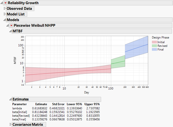
By default, the Piecewise Weibull NHPP report shows the estimated MTBF plot. The phases are differentiated with different colors. The Estimates and Covariance Matrix reports are shown below the plot.
Figure 10.18 Piecewise Weibull NHPP Report
MTBF Plot
The MTBF plot and the Estimates report appear by default when the Piecewise Weibull NHPP option is chosen (Figure 10.18). When Time to Event Format is used, the axes are logarithmically scaled. For more information about the plot, see MTBF Plot.
Estimates
The Estimates report gives estimates of the model parameters. Note that only the estimate for the value of λ corresponding to the first phase is given. In the piecewise model, the cumulative events at the end of one phase must match the number at the beginning of the subsequent phase. Because of these constraints, the estimate of λ for the first phase and the estimates of the βs determine the remaining λs.
The method used to calculate the estimates, their standard errors, and the confidence limits is similar to that used for the simple Crow-AMSAA model. See Parameter Estimates for Crow-AMSAA Models. The likelihood function reflects the additional parameters and the constraints on the cumulative numbers of events.
Covariance Matrix
Estimated covariance matrix for the estimates of the parameters of the fitted model. This report is closed by default.
Piecewise Weibull NHPP Options
This section describes the options available in the Piecewise Weibull NHPP red triangle menu.
Show MTBF Plot
This option shows or hides the MTBF plot. See MTBF Plot.
Show Intensity Plot
The Intensity plot shows the estimated intensity function and confidence bounds over the design phases. The intensity function is generally discontinuous at a phase transition. Color coding facilitates differentiation of phases. If Time to Event Format is used, the axes are logarithmically scaled. See Show Intensity Plot.
Show Cumulative Events Plot
The Cumulative Events plot shows the estimated cumulative number of events, along with confidence bounds, over the design phases. The model requires that the cumulative events at the end of one phase match the number at the beginning of the subsequent phase. Color coding facilitates differentiation of phases. If Time to Event Format is used, the axes are logarithmically scaled. See Show Cumulative Events Plot.
Show Profilers
Three profilers are displayed, showing estimated MTBF, Failure Intensity, and Cumulative Events. These profilers do not use logarithmic scaling. For more information about interpreting and using these profilers, see the section Show Profilers.
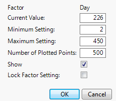
It is important to note that, due to the default resolution of the profiler plot, discontinuities are not displayed clearly in the MTBF or Failure Intensity Profilers. In the neighborhood of a phase transition, the profiler trace shows a nearly vertical, but slightly sloped, line; this line represents a discontinuity (Figure 10.19). Such a line at a phase transition should not be used for estimation. You can obtain a higher-resolution display making these lines appear more vertical as follows. Press Ctrl while clicking in the profiler plot, and then enter a larger value for Number of Plotted Points in the window. (See Figure 10.20, where we have specified 500 as the Number of Plotted Points.)
Figure 10.19 Profilers
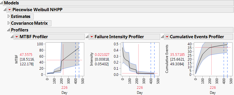
Figure 10.20 Factor Settings Window