Power Analysis
The Power Analysis outline calculates the power of tests for the parameters in your model. Power is the probability of detecting an active effect of a given size. The Power Analysis outline helps you evaluate the ability of your design to detect effects of practical importance. The higher your power, the more likely you are to detect significant effects assuming your coefficient and RMSE assumptions are correct. Power depends on the number of runs, the significance level, and the estimated error variation. In particular, you can determine if additional runs are necessary.
This section covers the following topics:
• Tests for Individual Parameters
• Tests for Categorical Effects with More Than Two Levels
• Design and Anticipated Responses Outline
• Power Analysis for Coffee Experiment
Power Analysis Overview
Power is calculated for the effects listed in the Model outline. These include continuous, discrete numeric, categorical, blocking, mixture, and covariate factors. The tests are for individual model parameters and for whole effects. For more information on how power is calculated, see Power Calculations in the Technical Details section.
Power is the probability of rejecting the null hypothesis of no effect at specified values of the model parameters. In practice, your interest is not in the values of the model parameters, but in detecting differences in the mean response of practical importance. In the Power Analysis outline, you can compute Anticipated Responses for specified values of the Anticipated Coefficients. This helps you to determine the coefficient values associated with the differences you want to detect in the mean response.
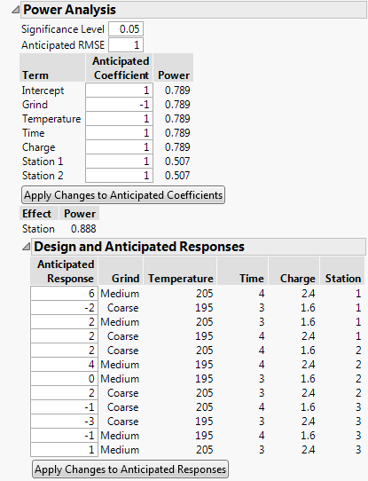
Figure 15.14 shows the Power Analysis outline for the design in the Coffee Data.jmp sample data table, found in the Design Experiment folder. The model specified in the Model script is a main effects only model.
Figure 15.14 Power Analysis for Coffee Data.jmp
In the Power Analysis outline, you can:
• Specify coefficient values that reflect differences that you want to detect. You enter these as Anticipated Coefficients in the top part of the outline.
• Specify anticipated response values and apply these to determine the corresponding Anticipated Coefficients. You specify Anticipated Responses in the Design and Anticipated Responses panel.
Power Analysis Details
Specify values for the Significance Level and Anticipated RMSE. These are used to calculate the power of the tests for the model parameters.
Significance Level
The probability of rejecting the hypothesis of no effect, if it is true. The power calculations update immediately when you enter a value.
Anticipated RMSE
An estimate of the square root of the error variation. The power calculations update immediately when you enter a value.
The top portion of the Power Analysis report opens with default values for the Anticipated Coefficients (Figure 15.14). The default values are based on Delta. See Advanced Options > Set Delta for Power.
Note: If the design is supersaturated, meaning that the number of parameters to be estimated exceeds the number of runs, the anticipated coefficients are set to 0.
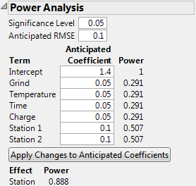
Figure 15.15 shows the top portion of the Power Analysis report where values have been specified for the Anticipated Coefficients. These values reflect the differences you want to detect.
Figure 15.15 Possible Specification of Anticipated Coefficients for Coffee Data.jmp
Tests for Individual Parameters
The Term column contains a list of model terms. For each term, the Anticipated Coefficient column contains a value for that term. The value in the Power column is the power of a test that the coefficient for the term is 0 if the true value of the coefficient is given by the Anticipated Coefficient.
Term
The model term associated with the coefficient being tested.
Note: The order in which model terms appear in the Power Analysis report may not be identical to their order in the Parameter Estimates report obtained using Standard Least Squares. This difference can only occur when the model contains an interaction with more than one degree of freedom.
Anticipated Coefficient
A value for the coefficient associated with the model term. This value is used in the calculations for Power. These values are also used to calculate the Anticipated Response column in the Design and Anticipated Responses outline. When you set a new value in the Anticipated Coefficient column, click Apply Changes to Anticipated Coefficients to update the Power and Anticipated Response columns.
Note: The anticipated coefficients have default values of 1 for continuous effects. They have alternating values of 1 and –1 for categorical effects. You can specify a value for Delta be selecting Advanced Options > Set Delta for Power from the red triangle menu. If you change the value of Delta, the values of the anticipated coefficients are updated so that their absolute values are one-half of Delta. See Advanced Options > Set Delta for Power.
Power
Probability of rejecting the null hypothesis of no effect when the true coefficient value is given by the specified Anticipated Coefficient. For a coefficient associated with a numeric factor, the change in the mean response (based on the model) is twice the coefficient value. For a coefficient associated with a categorical factor, the change in the mean response (based on the model) across the levels of the factor equals twice the absolute value of the anticipated coefficient.
Calculations use the specified Significance Level and Anticipated RMSE. For more information about the power calculation, see Power for a Single Parameter in the Technical Details section.
Apply Changes to Anticipated Coefficients
When you set a new value in the Anticipated Coefficient column, click Apply Changes to Anticipated Coefficients to update the Power and Anticipated Response columns.
Tests for Categorical Effects with More Than Two Levels
If your model contains a categorical effect with more than two levels, then the following columns appear below the Apply Changes to Anticipated Coefficients button:
Effect
The categorical effect.
Power
The power calculation for a test of no effect. The null hypothesis for the test is that all model parameters corresponding to the effect are zero. The difference to be detected is defined by the values in the Anticipated Coefficient column that correspond to the model terms for the effect. The power calculation reflects the differences in response means determined by the anticipated coefficients.
Calculations use the specified Significance Level and Anticipated RMSE. For more information about the power calculation, see Power for a Categorical Effect in the Technical Details section.
Design and Anticipated Responses Outline
The Design and Anticipated Responses outline shows the design preceded by an Anticipated Response column. Each entry in the first column is the Anticipated Response corresponding to the design settings. The Anticipated Response is calculated using the Anticipated Coefficients.
Figure 15.16 shows the Design and Anticipated Responses outline corresponding to the specification of Anticipated Coefficients given in Figure 15.15.
Figure 15.16 Anticipated Responses for Coffee Data.jmp
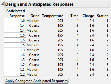
In the Anticipated Response column, you can specify a value for each setting of the factors. These values reflect the differences you want to detect.
Click Apply Changes to Anticipate Responses to update both the Anticipated Coefficient and Power columns.
Anticipated Response
The response value obtained using the Anticipated Coefficient values as coefficients in the model. When the outline first appears, the calculation of Anticipated Response values is based on the default values in the Anticipated Coefficient column. When you set new values in the Anticipated Response column, click Apply Changes to Anticipated Responses to update the Anticipated Coefficient and Power columns.
Design
The columns to the right of the Anticipated Response column show the factor settings for all runs in your design.
Apply Changes to Anticipated Responses
When you set new values in the Anticipated Response column, click Apply Changes to Anticipated Responses to update the Anticipated Coefficient and Power columns.
Power Analysis for Coffee Experiment
Consider the design in the Coffee Data.jmp data table. Suppose that you are interested in the power of your design to detect effects of various magnitudes on Strength. Recall that Grind is a two-level categorical factor, Temperature, Time, and Charge are continuous factors, and Station is a three-level categorical (blocking) factor.
In this example, ignore the role of Station as a blocking factor. You are interested in the effect of Station on Strength. Since Station is a three-level categorical factor, it is represented by two terms in the Parameters list: Station 1 and Station 2.
Specifically, you are interested the probability of detecting the following changes in the mean Strength:
• A change of 0.10 units as you vary Grind from Coarse to Medium.
• A change of 0.10 units or more as you vary Temperature, Time, and Charge from their low to high levels.
• An increase due to each of Stations 1 and 2 of 0.10 units beyond the overall anticipated mean. This corresponds to a decrease due to Station 3 of 0.20 units from the overall anticipated mean.
You set 0.05 as your Significance Level. Your estimate of the standard deviation of Strength for fixed design settings is 0.1 and you enter this as the Anticipated RMSE.
Figure 15.17 shows the Power Analysis node with these values entered. Specifically, you specify the Significance Level, Anticipated RMSE, and the value of each Anticipated Coefficient.
When you click Apply Changes to Anticipated Coefficients, the Anticipated Response values are updated to reflect the model you have specified.
Figure 15.17 Power Analysis Outline with User Specifications in Anticipated Coefficients Panel
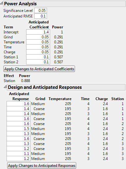
Recall that Temperature is a continuous factor with coded levels of -1 and 1. Consider the test whose null hypothesis is that Temperature has no effect on Strength. Figure 15.17 shows that the power of this test to detect a difference of 0.10 (=2*0.05) units across the levels of Temperature is only 0.291.
Now consider the test for the whole Station effect, where Station is a three-level categorical factor. Consider the test whose null hypothesis is that Station has no effect on Strength. This is the usual F test for a categorical factor provided in the Effect Tests report when you run Analyze > Fit Model. See Effect Tests in Fitting Linear Models.
The Power of this test is shown directly beneath the Apply Changes to Anticipated Coefficients button. The entries under Anticipated Coefficients for the model terms Station 1 and Station 2 are both 0.10. These settings imply that the effect of both stations is to increase Strength by 0.10 units above the overall anticipated mean. For these settings of the Station 1 and Station 2 coefficients, the effect of Station 3 on Strength is to decrease it by 0.20 units from the overall anticipated mean. Figure 15.17 shows that the power of the test to detect a difference of at least this magnitude is 0.888.