Saved Formulas
This section gives the derivation of formulas saved by Score Options > Save Formulas. The formulas depend on the Discriminant Method.
For each group defined by the categorical variable X, observations on the covariates are assumed to have a p-dimensional multivariate normal distribution, where p is the number of covariates. The notation used in the formulas is given in Table 5.2.
|
p |
number of covariates |
|
T |
total number of groups (levels of X) |
|
t = 1,..., T |
subscript to distinguish groups defined by X |
|
nt |
number of observations in group t |
|
n = n1 + n2 + ... + nT |
total number of observations |
|
y |
p by 1 vector of covariates for an observation |
|
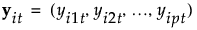
ith observation in group t, consisting of a vector of p covariates |
|
p by 1 vector of means of the covariates y for observations in group t |
|
ybar |
p by 1 vector of means for the covariates across all observations |
|
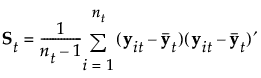
estimated (p by p) within-group covariance matrix for group t |
|
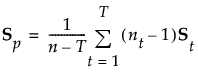
estimated (p by p) pooled within covariance matrix |
|
qt |
prior probability of membership for group t |
|
p(t|y) |
posterior probability that y belongs to group t |
|
|A| |
determinant of a matrix A |

Linear Discriminant Method
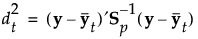
In linear discriminant analysis, all within-group covariance matrices are assumed equal. The common covariance matrix is estimated by Sp. See Table 5.2 for notation.
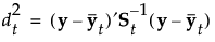
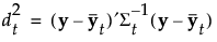
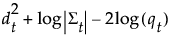
The Mahalanobis distance from an observation y to group t is defined as follows:
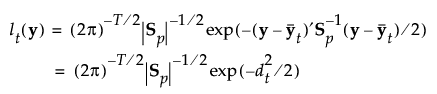
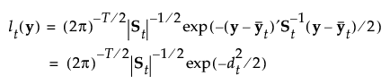
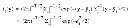
The likelihood for an observation y in group t is estimated as follows:
Note that the number of parameters that must be estimated for the pooled covariance matrix is p(p+1)/2 and for the means is Tp. The total number of parameters that must be estimated is p(p+1)/2 + Tp.
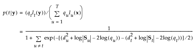
The posterior probability of membership in group t is given as follows:
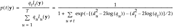
An observation y is assigned to the group for which its posterior probability is the largest.
The formulas saved by the Linear discriminant method are defined as follows:
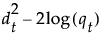
SqDist[0] |
|
|---|---|
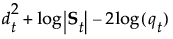
SqDist[<group t>] |
|
Prob[<group t>] |
|
Pred <X> | t for which p(t|y) is maximum, t = 1, ..., T |


Quadratic Discriminant Method
In quadratic discriminant analysis, the within-group covariance matrices are not assumed equal. The within-group covariance matrix for group t is estimated by St. This means that the number of parameters that must be estimated for the within-group covariance matrices is Tp(p+1)/2 and for the means is Tp. The total number of parameters that must be estimated is Tp(p+3)/2.
When group sample sizes are small relative to p, the estimates of the within-group covariance matrices tend to be highly variable. The discriminant score is heavily influenced by the smallest eigenvalues of the inverse of the within-group covariance matrices. See Friedman (1989). For this reason, if your group sample sizes are small compared to p, you might want to consider the Regularized method, described in Regularized Discriminant Method.
See Table 5.2 for notation. The Mahalanobis distance from an observation y to group t is defined as follows:
The likelihood for an observation y in group t is estimated as follows:
The posterior probability of membership in group t is the following:
An observation y is assigned to the group for which its posterior probability is the largest.
The formulas saved by the Quadratic discriminant method are defined as follows:
SqDist[<group t>] |
|
Prob[<group t>] |
|
Pred <X> | t for which p(t|y) is maximum, t = 1, ..., T |

Note: SqDist[<group t>] can be negative.
Regularized Discriminant Method
Regularized discriminant analysis allows for two parameters: λ and γ.
• The parameter λ balances weights assigned to the pooled covariance matrix and the within-group covariance matrices, which are not assumed equal.
• The parameter γ determines the amount of shrinkage toward a diagonal matrix.
This method enables you to leverage two aspects of regularization to bring stability to estimates for quadratic discriminant analysis. See Friedman (1989). See Table 5.2 for notation.
For the regularized method, the covariance matrix for group t is:

The Mahalanobis distance from an observation y to group t is defined as follows:
The likelihood for an observation y in group t is estimated as follows:
The posterior probability of membership in group t given by the following:

An observation y is assigned to the group for which its posterior probability is the largest.
The formulas saved by the Regularized discriminant method are defined below:
SqDist[<group t>] |
|
Prob[<group t>] |
|
Pred <X> | t for which p(t|y) is maximum, t = 1, ..., T |

Note: SqDist[<group t>] can be negative.
Wide Linear Discriminant Method
The Wide Linear method is useful when you have a large number of covariates and, in particular, when the number of covariates exceeds the number of observations (p > n). This approach centers around an efficient calculation of the inverse of the pooled within-covariance matrix Sp or of its transpose, if p > n. It uses a singular value decomposition approach to avoid inverting and allocating space for large covariance matrices.
The Wide Linear method assumes equal within-group covariance matrices and is equivalent to the Linear method if the number of observations equals or exceeds the number of covariates.
Wide Linear Calculation
See Table 5.2 for notation. The steps in the Wide Linear calculation are as follows:
1. Compute the T by p matrix M of within-group sample means. The (t,j)th entry of M, mtj, is the sample mean for members of group t on the jth covariate.
2. For each covariate j, calculate the pooled standard deviation across groups. Call this sjj.
3. Denote the diagonal matrix with diagonal entries sjj by Sdiag.
4. Center and scale values for each covariate as follows:
– Subtract the mean for the group to which the observation belongs.
– Divide the difference by the pooled standard deviation.
Using notation, for an observation i in group t, the group-centered and scaled value for the jth covariate is:
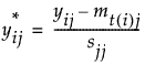
The notation t(i) indicates the group t to which observation i belongs.
5. Denote the matrix of  values by Ys.
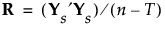
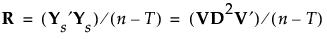
6. Denote the pooled within-covariance matrix for the group-centered and scaled covariates by R. The matrix R is given by the following:
7. Apply the singular value decomposition to Ys:
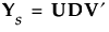
where U and V are orthonormal and D is a diagonal matrix with positive entries (the singular values) on the diagonal. See The Singular Value Decomposition in the Statistical Details section.
Then R can be written as follows:
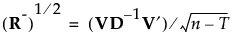
8. If R is of full rank, obtain R-1/2 as follows:
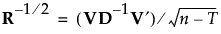
where D-1 is the diagonal matrix whose diagonal entries are the inverses of the diagonal entries of D.
If R is not of full rank, define a pseudo-inverse for R as follows:
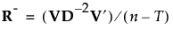
Then define the inverse square root of R as follows:
9. If R is of full rank, it follows that R- = R-1. So, for completeness, the discussion continues using pseudo-inverses.
Define a p by p matrix Ts as follows:
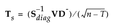
Then:
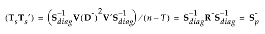
where S-p is a generalized inverse of the pooled within-covariance matrix for the original data that is calculated using the SVD.
Mahalanobis Distance
The formulas for the Mahalanobis distance, the likelihood, and the posterior probabilities are identical to those in Linear Discriminant Method. However, the inverse of Sp is replaced by a generalized inverse computed using the singular value decomposition.
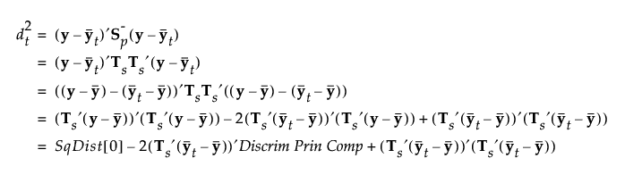
When you save the formulas, the Mahalanobis distance is given in terms of the decomposition. For an observation y, the squared distance to group t is the following, where SqDist[0] and Discrim Prin Comp in the last equality are defined in Saved Formulas:
Saved Formulas
The formulas saved by the Wide Linear discriminant method are defined as follows:
Discrim Data Matrix | Vector of observations on the covariates |
Discrim Prin Comp | The data transformed by the principal component scoring matrix, which renders the data uncorrelated within groups. Given by |
SqDist[0] |
|
SqDist[<group t>] | The Mahalanobis distance from the from observation to the group centroid. See Mahalanobis Distance. |
Prob[<group t>] |
|
Pred <X> | t for which p(t|y) is maximum, t = 1, ..., T |
 , where
  is a
is a 
 , given in