Simulate Responses
When you click Make Table to create your design table, the Simulate Responses option does the following for each response:
• It adds random response values to the response column in your design table.
• It adds a new a column containing a simulation model formula to the design table. The formula and values are based on the model that is specified in the design window.
A Model window opens where you can specify parameter values and select a response distribution for simulation. When you click Apply in the Model window, each column containing a simulation model formula is updated.
Control Window
Figure 4.27 shows the Model window for a design with one continuous factor (X1) and one three-level categorical factor (X2). Notice that X2 is represented by two model terms.
Figure 4.27 Simulate Responses Control Window
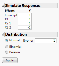
The initial window shows values for the coefficients of either 1 or -1, and a Normal distribution with error standard deviation equal to 1. If you have set Anticipated Coefficients as part of Power Analysis under Design Evaluation in the DOE window, then the default values in the Simulate Responses outline are the values that you specified as Anticipated Coefficients and Anticipated RMSE (Error Std) in the Power Analysis outline. If it is not possible to fit the model specified in the data table’s Model script, the intercept and coefficients have default values of 0.
Simulate Responses
To specify a model for simulated values, do the following:
1. For each term in the list of Effects, enter coefficients for the linear model used to simulate the response values. These define a linear function, L(x, β) = x‘β. See the Simulate Responses outline in Figure 4.27:
– The vector x consists of the terms that define the effects listed under Effects.
– The vector β is the vector of model coefficients that you specify under Y.
2. Under Distribution, select a response distribution.
3. Click Apply. A <Y> Simulated column containing simulated values and their formula is added to the design table, where Y is the name of the response column.
Distribution
Choose from one of the following distributions in the Simulate Responses window:
Normal
Simulates values from a normal distribution. Enter a value for Error σ, the standard deviation of the normal error distribution. If you have designated factors to have Changes of Hard in the Factors outline, you can enter a value for Whole Plots σ, the whole plot error. If you have designated factors to have Changes of Hard and Very Hard, you can enter values for both the subplot and whole plot errors. When you click Apply, random values and a formula containing a random response vector based on the model are entered in the column <Y> Simulated.
Binomial
Simulates values from a binomial distribution. Enter a value for N, the number of trials. Random integer values are generated according to a binomial distribution based on N trials with probability of success 1/(1 + exp(-L(x, β)). When you click Apply, random values and their formula are entered in the column <Y> Simulated. A column called N Trials that contains the value N is also added to the data table.
Poisson
Simulates random integer values according to a Poisson distribution with parameter exp((L(x, β)). When you click Apply, random values and their formula are entered in the column <Y> Simulated.
Note: You can set a preference to simulate responses every time you click Make Table. To do so, select File > Preferences > Platforms > DOE. Select Simulate Responses.