Simulation of Confidence Limits for a Nonnormal Process Ppk
In this example, you first perform a capability analysis for the three nonnormal variables in Tablet Measurements.jmp. You then use Simulate to find confidence limits for the nonconformance percentage for the variable Purity.
Nonnormal Capability Analysis
If you prefer not to follow the steps below, you can obtain the results in this section by running the Process Capability table script in Tablet Measurements.jmp.
1. Select Help > Sample Data Library and open Tablet Measurements.jmp.
2. Select Analyze > Quality and Process > Process Capability.
3. Select Weight, Thickness, and Purity and click Y, Process.
4. Select Weight, Thickness, and Purity in the Cast Selected Columns into Roles list on the right.
5. Open the Distribution Options outline.
6. From the Distribution list, select Best Fit.
7. Click Set Process Distribution.
The &Dist(Best Fit) suffix is added to each column name in the list on the right.
8. Click OK.
A Capability Index Plot appears, showing the Ppk values. Note that only the Thickness variable appears above the line that denotes Ppk = 1. Purity is nearly on the line. Although the number of measurements, 250, seems large, the estimated Ppk value is still quite variable. For this reason, you construct a confidence interval for the true Purity Ppk value.
Note: Because a Goal Plot is not shown, you can conclude that a normal distribution fit was not the best fit for any of the three variables.
9. Click the Process Capability red triangle and select Individual Detail Reports.
The best fits are as follows:
– Weight: Lognormal
– Thickness: SHASH
– Purity: Weibull
Construct the Simulation Column
To use the Simulate utility to estimate Ppk confidence limits, you need to construct a simulation formula that reflects the fitted Weibull distribution. If you prefer not to follow the steps below, you can obtain the results in this section by running the Add Simulation Column table script.
1. Scroll to the Purity (Weibull) Capability report and find the Parameter Estimates report.
Figure 7.27 Weibull Parameter Estimates for Purity
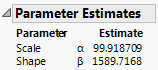
These are the parameter estimates for the best fitting distribution, which is Weibull.
2. In the Tablet Measurements.jmp sample data table, select Cols > New Columns.
3. Next to Column Name, enter Simulated Purity.
4. From the Column Properties list, select Formula.
5. In the formula editor, select Random > Random Weibull.
6. The placeholder for beta is selected. Click the insertion element (^).
Figure 7.28 Formula Editor for Simulated Purity Column
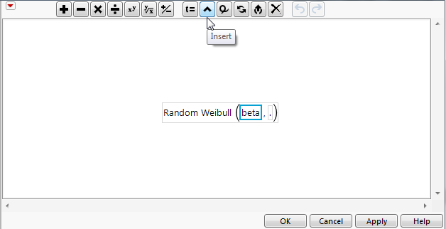
This adds a placeholder for the parameter alpha.
7. Right-click in the Parameter Estimates report table and select Make into Data Table.
8. Copy the entry in Row 2 in the Estimate column (1589.7167836).
9. In the formula editor window, select the placeholder for beta in the Random Weibull formula and paste 1589.7167836 into the placeholder for beta.
10. In the data table that you created from the Parameter Estimates report, copy the entry in Row 1 in the Estimate column (99.918708989).
11. In the formula editor window, select the placeholder for alpha in the Random Weibull formula and paste 99.918708989 into the placeholder for alpha.
Figure 7.29 Completed Formula Window
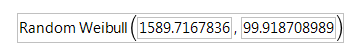
12. Click OK in the formula editor window.
13. From the Column Properties list, select Spec Limits.
14. Next to Lower Spec Limit, type 99.5.
15. Click OK in the New Column window.
The Simulated Purity column contains a formula that simulates values from the best-fitting distribution.
Simulate Confidence Intervals for Purity Ppk and Expected Percent Nonconforming
When you use Simulate, the entire analysis is run the number of times that you specify. To shorten the computing time, you can minimize the computational burden by running only the required analysis. In this example, because you are interested only in Purity with a fitted Weibull distribution, you perform only this analysis before running Simulate.
Note: If you do not care about computing time, you can use the same report you created in the previous section and start with step 7.
1. In the Process Capability report, click the Process Capability red triangle and select Relaunch Dialog.
2. (Optional) Close the Process Capability report.
3. In the launch window, from the Cast Selected Columns into Roles list, select Weight&Dist(Lognormal) and Thickness&Dist(Johnson).
4. Click Remove.
5. Click OK.
6. Click the Process Capability red triangle and select Individual Detail Reports.
Both Ppk and Ppl values are provided, but they are identical because Purity has only a lower specification limit.
7. In the Overall Sigma Capability report, right-click the Estimate column and select Simulate.
In the Column to Switch Out list, make sure Purity is selected. In the Column to Switch In list, make sure Simulated Purity is selected.
8. Next to Number of Samples, type 500.
Note: The next step is not required. However, it ensures that you obtain exactly the simulated values shown in this example.
9. (Optional) Next to Random Seed, type 12345.
10. Click OK.
The calculation might take several seconds. A data table entitled Process Capability Simulate Results (Estimate) appears. The Ppk and Ppl columns in this table each contain 500 values calculated based on the Simulated Purity formula. The first row, which is excluded, contains the values for Purity obtained in your original analysis. Because Purity has only a lower specification limit, the Ppk values are identical to the Ppl values.
11. In the Process Capability Simulate Results (Estimate) data table, click the green triangle next to the Distribution script.
Figure 7.30 Distribution of Simulated Ppk Values for Purity
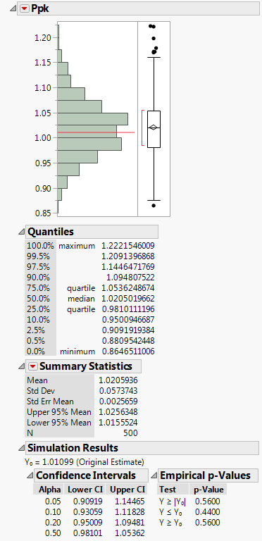
Note: Your values may vary slightly from what is shown, depending on the decimal precision of the parameters in the Simulated Purity column formula.
Two Distribution reports are shown, one for Ppk and one for Ppl. But Purity has only a lower specification limit, so that the Ppk and Ppl values are identical. For this reason, the Distribution reports are identical.
The Simulation Results report shows that a 95% confidence interval for Ppk is 0.909 to 1.145. The true Ppk value could be above 1.0, which would place Purity above the Ppk = 1 line in the Capability Index Plot you constructed in Nonnormal Capability Analysis.
12. In the Process Capability report, right-click the Expected Overall % column in the Nonconformance report and select Simulate.
In the Column to Switch Out list, make sure Purity is selected. In the Column to Switch In list, make sure Simulated Purity is selected.
13. Next to Number of Samples, enter 500.
14. (Optional) Next to Random Seed, enter 12345.
15. Click OK.
The calculation might take several seconds. A data table entitled Process Capability Simulate Results (Expected Overall %) appears. Because Purity has only a lower specification limit, the Below LSL values are identical to the Total Outside values.
16. In the Process Capability Simulate Results (Expected Overall %) data table, click the green triangle next to the Distribution script.
Figure 7.31 Distribution of Simulated Total Outside Values for Purity
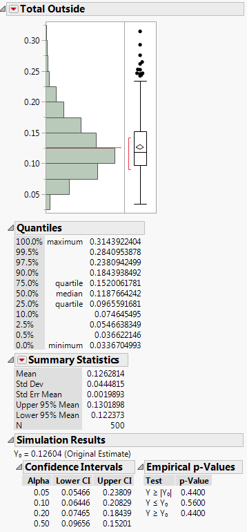
Note: Your values may vary slightly from what is shown, depending on the decimal precision of the parameters in the Simulated Purity column formula.
Again, two identical Distribution reports appear. The Simulation Results report shows that a 95% confidence interval for the Expected Overall % nonconforming is 0.055 to 0.238.