Split-Plot Experiment
Split-plot designs originated in agriculture, but are commonplace in manufacturing and engineering studies. In a split-plot experiment, hard-to-change factors are reset only between one whole plot and the next whole plot. The whole plot is divided into subplots, and the levels of the easy-to-change factors are randomly assigned to each subplot.
The example in this section is adapted from Kowalski, Cornell, and Vining (2002). You are interested in the effects of five factors on the thickness of vinyl that is used to make automobile seat covers. The response and factors in the experiment are described below:
• The response is the thickness of the vinyl that is produced. You want to maximize thickness. A lower limit for thickness values is 10.
• The whole plot factors are the rate of extrusion (extrusion rate) and the temperature (temperature) of drying. These are process variables and are hard to change.
• The subplot factors are three plasticizers whose proportions (m1, m2, and m3) sum to one. These factors are mixture components.
Your experimental budget allows for running 7 settings of these whole plot factors. For each whole plot, you can conduct 4 runs of the subplot factors. This gives you a total of 28 runs.
Create the Design
1. Select DOE > Custom Design.
2. Double-click Y under Response Name and type thickness.
Keep the default goal set to Maximize.
3. Enter a Lower Limit of 10.
To add factors manually, follow step 4 through step 11. Or, to load factors from a saved table, select Load Factors from the Custom Design red triangle. Open the Vinyl Factors.jmp sample data table, located in the Design Experiment folder. If you select Load Factors, skip step 4 through step 11.
4. Type 2 next to Add N Factors.
5. Click Add Factor > Continuous.
6. Rename these factors extrusion rate and temperature.
Keep the default Values of –1 and 1 for these two factors.
7. Click Easy and select Hard for both extrusion rate and temperature.
This defines extrusion rate and temperature to be whole plot factors.
8. Type 3 next to Add N Factors.
9. Click Add Factor > Mixture.
10. Rename the three mixture factors m1, m2, and m3.
Keep the default Values of 0 and 1 for those three factors.
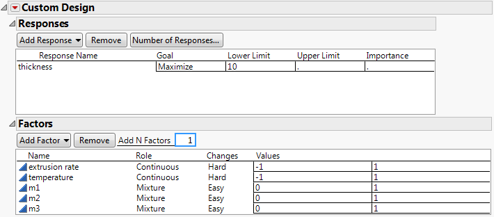
Figure 5.72 Responses and Factors Outlines
11. Click Continue.
12. Click Interactions > 2nd.
13. Click OK to dismiss the informative message.
Note that 3 is the default value for the Number of Whole Plots.
14. Type 7 next to Number of Whole Plots.
15. Type 28 next to User Specified.
Note: Setting the Random Seed in step 16 and Number of Starts in step 17 reproduces the exact results shown in this example. In constructing a design on your own, these steps are not necessary.
16. (Optional) Click the Custom Design red triangle, select Set Random Seed, type 12345, and click OK.
17. (Optional) Click the Custom Design red triangle, select Number of Starts, type 5, and click OK.
18. Click Make Design.
Figure 5.73 Design Outline
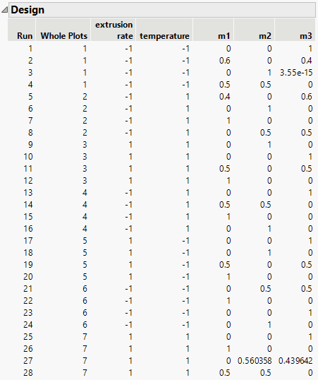
Note that the whole plot factors, extrusion rate and temperature, are reset seven times in accordance with the levels of the factor Whole Plots. Within each level of Whole Plots, the settings for the mixture ingredients, m1, m2, and m3, are assigned at random.
Analyze the Results
The Vinyl Data.jmp sample data table contains experimental results using a design created in a previous version of JMP.
1. Select Help > Sample Data Library and open Design Experiment/Vinyl Data.jmp.
This sample data table contains 28 runs and response values. The design settings in the table that you created using the Custom Design platform might differ from those used in the Vinyl Data.jmp design.
2. In the Table panel, click the green triangle next to the Model script.
Figure 5.74 Fit Model Window
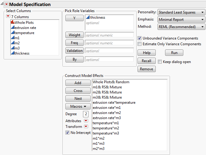
Notice the following in the Fit Model window:
– The factor Whole Plots has the Attribute called Random Effects (&Random). This specifies that the levels of Whole Plots are random realizations. They have an associated error term.
– The analysis method is REML (Recommended). This method is specified precisely because the model contains a random effect. For more information about REML models, see Restricted Maximum Likelihood (REML) Method in Fitting Linear Models.
Tip: In the Fit Model window, JMP Pro users can change the Personality to Mixed Model.
3. Click Run.
Figure 5.75 Split-Plot Analysis Results
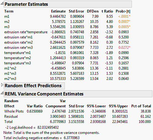
The Parameter Estimates report shows that the three mixture ingredients, as well as the extrusion rate*m3 interaction, are significant at the 0.05 level.
The REML Variance Component Estimates report indicates that the variance component associated with Whole Plots is 2.476748. This is 38.838% of the total variation. It follows that the error term associated with whole plot replication is smaller than the residual (or within-plot) error term.