The Two Basic Fitting Machines
An amazing fact about statistical fitting is that most of the classical methods reduce to using two simple machines, the spring and the pressure cylinder.
Springs
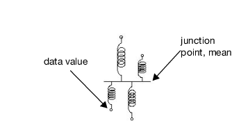
First, springs are the machine of fit for a continuous response model (Farebrother 1987). Suppose that you have n points and that you want to know the expected value (mean) of the points. Envision what happens when you lay the points out on a scale and connect them to a common junction with springs (Figure A.7). When you let go, the springs wiggle the junction point up and down and then bring it to rest at the mean. This is what must happen according to physics.
If the data are normally distributed with a mean at the junction point where springs are attached, then the physical energy in each point’s spring is proportional to the uncertainty of the data point. All you have to do to calculate the energy in the springs (the uncertainty) is to compute the sum of squared distances of each point to the mean.
To choose an estimate that attributes the least uncertainty to the observed data, the spring settling point is chosen as the estimate of the mean. That is the point that requires the least energy to stretch the springs and is equivalent to the least squares fit.
Figure A.7 Connect Springs to Data Points
That is how you fit one mean or fit several means. That is how you fit a line, or a plane, or a hyperplane. That is how you fit almost any model to continuous data. You measure the energy or uncertainty by the sum of squares of the distances that you must stretch the springs.
Statisticians put faith in the normal distribution because it is the one that requires the least faith. It is, in a sense, the most random. It has the most non-informative shape for a distribution. It is the one distribution that has the most expected uncertainty for a given variance. It is the distribution whose uncertainty is measured in squared distance. In many cases it is the limiting distribution when you have a mixture of distributions or a sum of independent quantities. It is the distribution that leads to test statistics that can be measured fairly easily.
When the fit is constrained by hypotheses, you test the hypotheses by measuring this same spring energy. Suppose you have responses from four different treatments in an experiment, and you want to test if the means are significantly different. First, envision your data plotted in groups as shown in Figure A.8, but with springs connected to a separate mean for each treatment. Then exert pressure against the spring force to move the individual means to the common mean. Presto! The amount of energy that constrains the means to be the same is the test statistic that you need. That energy is the main ingredient in the F test for the hypothesis that tests whether the means are the same.
Figure A.8 A Oneway Plot for a Continuous Response Variable
Pressure Cylinders
What if your response is categorical instead of continuous? For example, suppose that the response is the country of origin for a sample of cars. For your sample, there are probabilities for the three response levels, American, European, and Japanese. You can set these probabilities for country of origin to some estimate and then evaluate the uncertainty in your data. This uncertainty is found by summing the negative logs of the probabilities of the responses given by the data. It is written as follows:
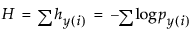
The idea of springs illustrates how a mean is fit to continuous data. When the response is categorical, statistical methods estimate the response probabilities directly and choose the estimates that minimize the total uncertainty of the data. The probability estimates must be nonnegative and sum to 1. You can picture the response probabilities as the composition along a scale whose total length is 1. For each response observation, load into its response area a gas pressure cylinder, such as a tire pump. Let the partitions between the response levels vary until an equilibrium of lowest potential energy is reached. The sizes of the partitions that result then estimate the response probabilities.
Figure A.9 shows what the situation looks like for a single category such as the medium size cars (see the mosaic column from Carpoll.jmp labeled medium in Figure A.10). Suppose there are thirteen responses (cars). The first level (American) has six responses, the next has two, and the last has five responses. The response probabilities become 6/13, 2/13, and 5/13, respectively, as the pressure against the response partitions balances out to minimize the total energy.
Figure A.9 Effect of Pressure Cylinders in Partitions
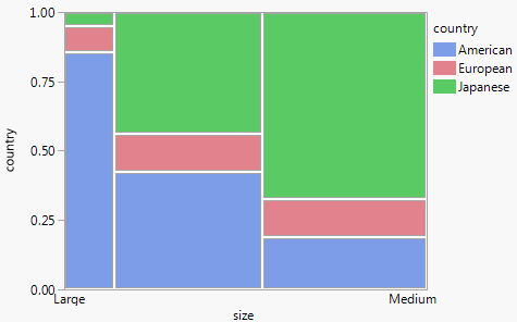
As with springs for continuous data, you can divide your sample by some factor and fit separate sets of partitions. Then test that the response rates are the same across the groups by measuring how much additional energy you need to push the partitions to be equal. Imagine the pressure cylinders for car origin probabilities grouped by the size of the car. The energy required to force the partitions in each group to align horizontally tests whether the variables have the same probabilities. Figure A.10 shows these partitions.
Figure A.10 A Mosaic Plot for Categorical Data