Analysis of Covariance with Equal Slopes Example
An analysis of variance model with a continuous regressor term is called an analysis of covariance. In the Drug.jmp sample data table, the column x is a covariate.
The covariate adds an additional term, x3i, to the model equation. The model analysis of covariance model is written this way:

There are two model effects: one is a nominal main effect involving two parameters, and the other is continuous covariate associated with one parameter.
1. Select Help > Sample Data Library and open Drug.jmp.
2. Select Analyze > Fit Model.
3. Select y and click Y.
4. Select both Drug and x and click Add.
5. Click Run.
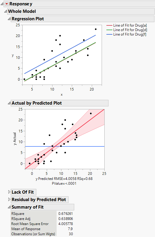
The Regression Plot in the report shows that you have fit a model with equal slopes (Figure 4.4). Compared to the main effects model (Drug effect only), RSquare increases from 22.8% to 67.6%. The Root Mean Square Error decreases from 6.07 to 4.0. As shown in Figure 4.4, the F test significance probability for the whole model decreases from 0.03 to less than 0.0001.
Figure 4.4 Analysis of Covariance for Drug Data
The drug data table contains replicated observations. For example, rows 1 and 9 both have Drug = a and x = 11. When fitting models, replicated observations can be used to construct a pure error estimate of variation. Another estimate of error can be constructed for unspecified functional forms of covariates, or interactions of nominal effects. These estimates form the basis for a lack of fit test. If the lack of fit error is significant, this indicates that there is some effect in your data not explained by your model.
The Lack of Fit report shows the results of this test for the drug data. The lack of fit error is not significant, as seen by the Prob > F value of 0.7507.
The covariate, x, accounts for much of the variation in the response previously accounted for by the Drug variable. Thus, even though the model is fit with much less error, the Drug effect is no longer significant. The significance of Drug observed in the main effects model appears to be explained by the covariate.
The least squares means in the covariance model differ from the ordinary means. This is because they are adjusted for the effect of x, the covariate, on the response, y. The least squares means are values predicted for each of the three levels of Drug, when the covariate, x, is held at some neutral value. The neutral value is chosen to be the mean of the covariate, which is 10.7333.
The least squares means are calculated using the parameter estimates given in the Parameter Estimates report:
Prediction Expression:
-2.696 - 1.185*Drug[a] - 1.0761*Drug[d] + 0.98718*x
For a:
-2.696 - 1.185*(1) -1.0761*(0) + 0.98718*(10.7333) = 6.71
For d:
-2.696 - 1.185*(0) -1.0761*(1) + 0.98718*(10.7333) = 6.82
For f:
-2.696 - 1.185*(-1) -1.0761*(-1) + 0.98718*(10.7333) = 10.16
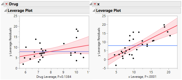
Figure 4.5 shows a leverage plot for each effect. Because the covariate is significant, the leverage values for Drug are dispersed somewhat from their least squares means.
Figure 4.5 Comparison of Leverage Plots for Drug Test Data

