Example of Informative Missing
In this example, you construct a decision tree model to predict if a customer is a credit risk. Since your data set contains missing values, you also explore the effectiveness of the Informative Missing option.
Launch the Partition Platform
1. Select Help > Sample Data Library and open Equity.jmp.
2. Select Analyze > Predictive Modeling > Partition.
3. Select BAD and click Y, Response.
4. Select LOAN through DEBTINC and click X, Factor.
5. Click OK.
Create the Decision Tree and ROC Curve with Informative Missing
1. Press Shift and click Split.
2. Enter 5 for the number of splits and click OK.
3. Click the red triangle next to Partition for BAD and select ROC Curve.
4. Click the red triangle next to Partition for BAD and select Save Columns > Save Prediction Formula.
The columns Prob(BAD==Good Risk) and Prob(BAD==Bad Risk) contain the formulas that Informative Missing utility uses to classify the credit risk of future loan applicants. You are interested in how this model performs in comparison to a model that does not use informative missing.
Create the Decision Tree and ROC Curve without Informative Missing
1. Click the red triangle next to Partition for BAD and select Redo > Relaunch Analysis
2. De-select Informative Missing.
3. Click OK and repeat the steps in Create the Decision Tree and ROC Curve with Informative Missing.
The columns Prob(BAD==Good Risk) 2 and Prob(BAD==Bad Risk) 2 contain the formulas that do not use the informative missing utility.
Compare the ROC Curves
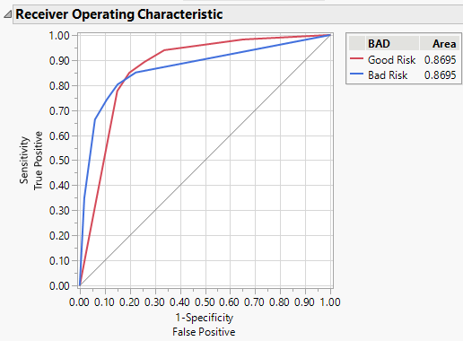
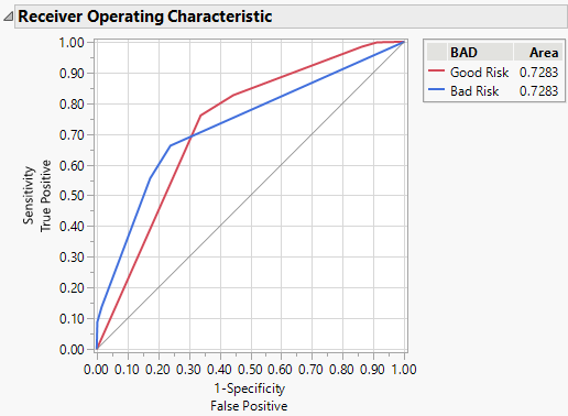
Visually compare the ROC curves from the two models. The model at left is with Informative Missing, and the model at right is without Informative Missing.
Figure 4.23 ROC Curves for Models with (Left) and without (Right) Informative Missing
The area under the curve (AUC) for the model with informative missing (0.8695) is higher than the AUC for the model without informative missing (0.7283). Because there are only two levels for the response, the ROC curves for each model are reflections of one another and the AUCs are equal.
Note: Your AUC can differ from that shown for the model without informative missing. When informative missing is not used, the assignment of missing rows to sides of a split is random. Rerunning the analysis can result in slight differences in results.
Use the Model Comparison Platform
Next, compare the models using the Model Comparison platform to compare the two sets of formulas that you created in step 4 and step 3.
1. Select Analyze > Predictive Modeling > Model Comparison.
2. Select Prob(BAD==Good Risk), Prob(BAD==Bad Risk), Prob(BAD==Good Risk) 2, and Prob(BAD==Bad Risk) 2 and click Y, Predictors.
The first pair of formula columns contains the formulas from the model with informative missing. The second pair of formula columns contains the formulas from the model without informative missing.
3. Click OK.
Figure 4.24 Measures of Fit from Model Comparison
The Measures of Fit report shows that the first model, which was fit with informative missing, performs better than the second model, which was not fit with informative missing. The first model has higher RSquare values as well as a lower RMSE value and a lower Misclassification Rate. These findings align the ROC curves comparison.
Note: Again, your results can differ due to the random differences when Informative Missing is not used.


