Example of Stacking Data for a Oneway Analysis
When your data are in a format other than a JMP data table, sometimes they are arranged so that a row contains information for multiple observations. To analyze the data in JMP, you must import the data and restructure it so that each row of the JMP data table contains information for a single observation. For example, suppose that your data are in a spreadsheet. The data for parts produced on three production lines are arranged in three sets of columns. In your JMP data table, you need to stack the data from the three production lines into a single set of columns so that each row represents the data for a single part.
Description and Goals
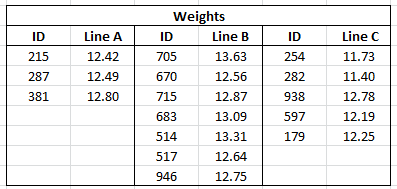
This example uses the file Fill Weights.xlsx, which contains the weights of cereal boxes randomly sampled from three different production lines. Figure 6.38 shows the format of the data.
• The ID columns contain an identifier for each cereal box that was measured.
• The Line columns contain the weights (in ounces) for boxes sampled from the corresponding production line.
Figure 6.38 Data Format
The target fill weight for the boxes is 12.5 ounces. Although you are interested in whether the three production lines are meeting the target, initially you want to see whether the three lines are achieving the same mean fill rate. You can use Oneway to test for differences among the mean fill weights.
To use the Oneway platform, you need to do the following:
1. Import the data into JMP. See Import the Data.
2. Reshape the data so that each row in the JMP data table reflects only a single observation. Reshaping the data requires that you stack the cereal box IDs, the line identifiers, and the weights into columns. See Stack the Data.
Import the Data
This example illustrates two ways to import data from Microsoft Excel into JMP. Select one method or explore both:
• Use the File > Open option to import data from a Microsoft Excel file using the Excel Import Wizard. See Import the Data Using the Excel Import Wizard. This method is convenient for any Excel file.
• Copy and paste data from Microsoft Excel into a new JMP data table. See Copy and Paste the Data from Excel. You can use this method with small data files.
For more information about how to import data from Microsoft Excel, see Import Microsoft Excel Files in Using JMP.
Import the Data Using the Excel Import Wizard
1. Select Help > Sample Data Library and open Fill Weights.xlsx located in the Samples/Import Data folder.
The file opens in the Excel Import Wizard.
2. Type 3 next to Column headers start on row.
In the Excel file, row 1 contains information about the table and row 2 is blank. The column header information starts on row 3.
3. Type 2 for Number of rows with column headers.
In the Excel file, rows 3 and 4 both contain column header information.
4. Click Import.
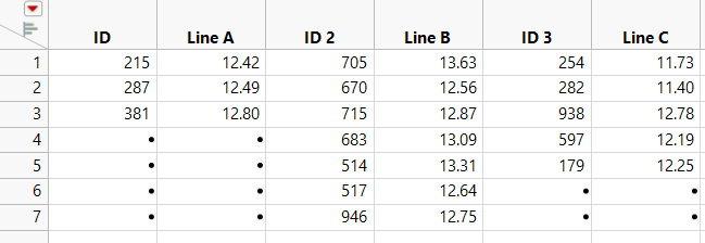
Figure 6.39 JMP Table Created Using Excel Import Wizard
The data are placed in seven rows and multiple IDs appear in each row. For each of the three lines, there are an ID and Weight column, giving a total of six columns.
Notice that the “Weights” part of the ID column name is unnecessary and misleading. You could rename the columns now, but it will be more efficient to rename the columns after you stack the data.
5. Proceed to Stack the Data.
Copy and Paste the Data from Excel
1. Open Fill Weights.xlsx in Microsoft Excel.
2. Select the data inside the table but exclude the unnecessary “Weights” heading.
3. Right-click and select Copy.
4. In JMP, select File > New > Data Table.
5. Select Edit > Paste with Column Names.
The Edit > Paste with Column Names option is used when your column names are included in the selection on the clipboard.
Figure 6.40 JMP Table Created Using Paste with Column Names
6. Proceed to Stack the Data.
Stack the Data
Use the Stack option to place one observation in each row of a new data table. For more information about the Stack option, see Stack Columns in Using JMP.
1. In the JMP data table, select Tables > Stack.
2. Select all six columns and click Stack Columns.
3. Select Multiple Series Stack.
You are stacking two series, ID and Line, so you do not change the Number of Series, which is set to 2 by default. The columns that contain the series are not contiguous. They alternate (ID, Line A, ID, Line B, ID, Line C). For this reason, you do not check Contiguous.
4. Deselect Stack By Row.
5. Select Eliminate Missing Rows.
6. Enter Stacked next to Output table name.
7. Click OK.
In the new data table, Data and Data 2 are columns containing the ID and Weight data.
8. Right-click the Label column heading and select Delete Columns.
The entries in the Label column were the column headings for the box IDs in the imported data table. These entries are not needed.
9. Rename each column by double-clicking on the column header:
– Data to ID
– Label 2 to Line
– Data 2 to Weight
10. In the Columns panel, click the icon to the left of ID and select Nominal.
Although ID is given as a number, it is an identifier and should be treated as nominal when modeling. This is not an issue in this example, but it is good practice to assign the appropriate modeling type to a column.
11. (Applies only if you imported the data from Excel using File > Open.) Do the following:
1. Click the Line column header to select the column and select Cols > Recode.
2. Click New Column and select In Place.
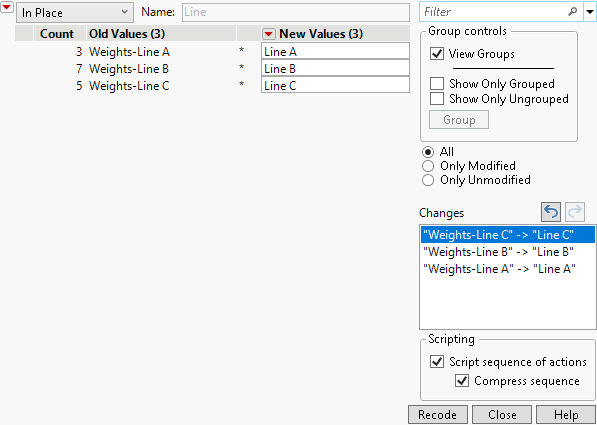
3. Change the values in the New Values column to match those in Figure 6.41 below.
Figure 6.41 Recode Column Values
4. Click Recode.
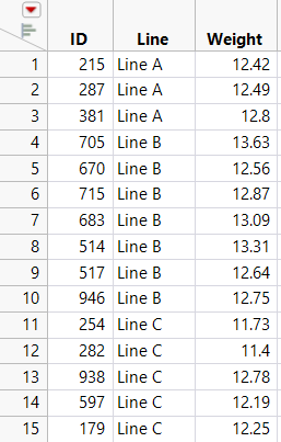
Your new data table is now properly structured for JMP analysis. Each row contains data for a single cereal box. The first column gives the box ID, the second gives the production line, and the third gives the weight of the box (Figure 6.42).
Figure 6.42 Recoded Data Table
Conduct the Oneway Analysis
This part of the example contains the following tasks:
• Conduct a Oneway Analysis of Variance to test for differences in the mean fill weights among the three production lines.
• Obtain Comparison Circles to explore which lines might differ.
• Label points by ID in case you want to reweigh or further examine their boxes.
Before beginning, verify that you are using the Stacked data table.
1. Select Analyze > Fit Y by X.
2. Select Weight and click Y, Response.
3. Select Line and click X, Factor.
4. Click OK.
5. Click the red triangle next to Oneway Analysis of Weight By Line and select Means/Anova.
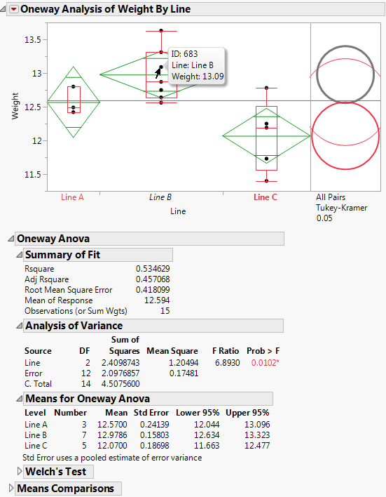
The mean diamonds in the plot show 95% confidence intervals for the production line means. The points that fall outside the mean diamonds might seem like outliers. However, they are not. To see this, add box plots to the plot.
6. Click the red triangle next to Oneway Analysis of Weight By Line and select Display Options > Box Plots.
All points fall within the box plots boundaries. Therefore, they are not outliers.
7. From the data table, in the Columns panel, right-click ID and select Label/Unlabel.
8. In the plot, hover over the points to see their ID values, as well as their Line and Weight data (Figure 6.43).
9. Click the red triangle next to Oneway Analysis of Weight By Line and select Compare Means > All Pairs, Tukey HSD.
Comparison circles appear in a panel to the right of the plot.
10. Click the bottom comparison circle.
Figure 6.43 Oneway Analysis of Weight by Line
In the Analysis of Variance report, the p-value of 0.0102 provides evidence that the means are not all equal. In the plot, the comparison circle for Line C is selected and appears red. Since the circle for Line B appears as thick gray, the mean for Line C differs from the mean for Line B at the 0.05 significance level. The means for Lines A and B do not show a statistically significant difference.
The mean diamonds shown in the plot span 95% confidence intervals for the means. The numeric bounds for the 95% confidence intervals are given in the Means for Oneway ANOVA report. Both of these indicate that the confidence intervals for Lines B and C do not contain the target fill weight of 12.5: Line B seems to overfill and Line C seems to underfill. For these two production lines, the underlying causes that result in off-target fill weights must be addressed.
