 Repeated Covariance Structures
This section gives the parameterizations for the following covariance structures:
• Unequal Variances Covariance Structure
• Unstructured Covariance Structure
• Compound Symmetry Covariance Structure
• Toeplitz Covariance Structure
• Antedependent Covariance Structure
 Unequal Variances Covariance Structure
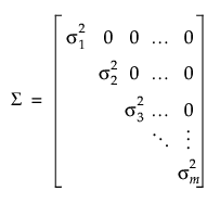
Here, the variance among observations taken at time j is:

The variances are allowed to differ across the levels of the repeated column. The covariances between observations at different levels are zero.
 Unstructured Covariance Structure
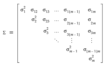
Here, the variance among observations taken at time j is:

The covariance between observations taken at times j and j′ is:

The variances are allowed to differ across the levels of the repeated column. The covariances between observations at different levels is unique.
 Compound Symmetry Covariance Structure
In JMP, a compound symmetry covariance structure is implemented using a mixed model with independent errors approach. Random effects are classified into two categories: G-side or R-side. See Searle et al. (1992).
The G-side random effects are associated with the design matrix for random effects. The R-side random effects are associated with residual error. Within-subject variance is part of the design structure and is modeled on the G-side. Between-subject variance falls into the residual structure and is modeled R-side. The variances in the independent structure are modeled in the following manner:
• The random effects G-side variance is modeled by sik ~ iid N(0, σs2).
• The R-side variance is modeled by eijk ~ iid N(0, σ 2).
Then the covariance matrix is defined as follows:
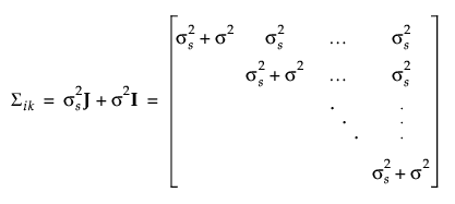
where J is a matrix consisting of 1s and I is an identity matrix.
Alternatively, all variance could be modeled on the R-side. Under the Gaussian assumption, this compound-symmetry covariance structure is equivalent to the independence model (Type=CS in SAS). This structure is available in JMP by using the Compound Symmetry structure in the repeated structure tab. Here, the correlation between pairs of repeated observations is the same regardless of the time difference between the observations. Thus, the correlation matrix can be specified as follows:
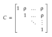
Using the Compound Symmetry structure in JMP also assumes a common variance,  , among observations taken at any time point. The covariance structure is then
  where
where

and
 .
.
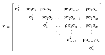
Here, ρ is the intra-class correlation coefficient and  is the residual variance. Another option is to use the Compound Symmetry Unequal Variances structure in JMP, which allows the variance to vary across time points. This leads to the following covariance matrix:
 AR(1) Covariance Structure
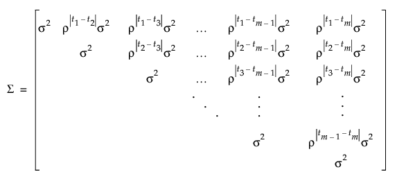
Here tj is the time of observation j. In this structure, observations taken at any given time have the same variance, σ2. The parameter ρ, where -1 < ρ < 1, is the correlation between two observations that are one unit of time apart. As the time difference between observations increases, their covariance decreases because ρ is raised to a higher power. In many applications, AR(1) provides an adequate model of the within subject correlation, providing more power without sacrificing Type I error control.
 Toeplitz Covariance Structure
In the Toeplitz structure, observations that are separated by a fixed number of time units have the same correlation. In contrast to the AR(1) correlation structure, the Toeplitz correlations at a fixed time difference are arbitrary. Denote the correlation for observations d units apart by ρd. The correlation matrix is defined as follows:
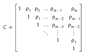
Two options in JMP use this correlation matrix:
• The Toeplitz structure assumes a common variance, σ2, for observations from any time point. The covariance structure is  .
.
• Alternatively, the Toeplitz Unequal Variances structure allows the variance to vary across time points:
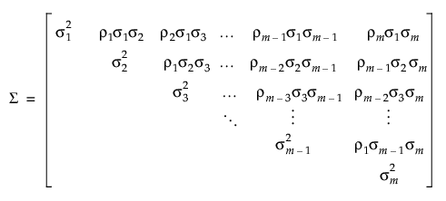
 Antedependent Covariance Structure
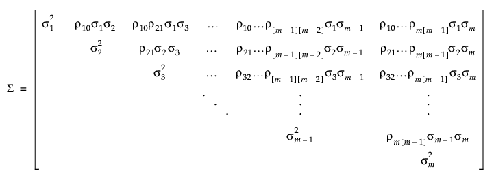
The antedependence model is a general model that is flexible and allows the correlation structure to change over time. In this model, the correlation between two observations at adjacent time points j - 1 and j is unique and is denoted ρj[j−1].
The correlation between pairs of observations at non-adjacent time points j and j′ is the product of all the adjacent correlations in between.

For example, the correlation between the pair of observations at time points j=2 and j′=6 would be ρ21ρ32ρ43ρ54.
The correlation matrix is defined as follows:
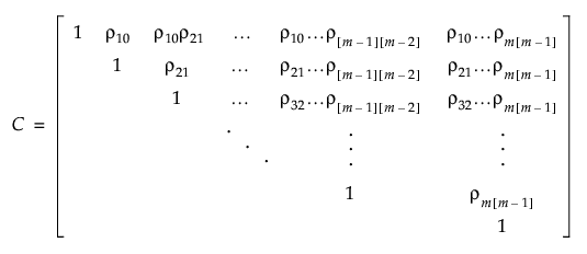
Two options in JMP use this correlation matrix:
• The Antedependent Equal Variance structure assumes equal variances across observation times while still allowing for the correlations to change. The variance among observations at any time is σ2 and the covariance matrix is  .
.
• The Antedependent structure allows the variance among observations at any given time to vary. Denote the variance among observations taken at time j is  . Then the covariance matrix is defined as follows:
