Comparisons with Overall Average
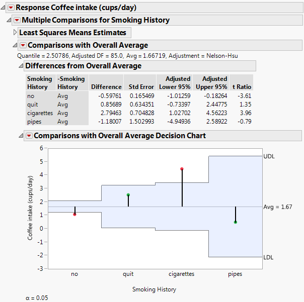
When you select the Multiple Comparisons option, you can choose the initial comparison to be with the overall average. This option compares the means for the specified levels specified to the overall mean for these levels. It displays a table showing confidence intervals for differences from the overall mean and a chart showing decision limits. The method used to make the comparisons is called analysis of means (ANOM) (Nelson et al. 2005). ANOM is a multiple comparison procedure that controls the joint error rate for all pairwise comparisons to the overall mean. See Figure 3.55 for a report based on the Lipid Data.jmp sample data table.
ANOM might appear similar to analysis of variance. However, it is fundamentally different in that it identifies levels with means that differ from the overall mean for all levels. In contrast, analysis of variance tests for differences in the means themselves.
At the top of the Comparisons with Overall Average report, you find:
Quantile
The value of Nelson’s h statistic used in constructing the decision limits.
Adjusted DF
The degrees of freedom used in constructing the decision limits.
Avg
The average mean. For least squares estimates, the average mean is a weighted average of the group least squares means. This weighted average represents the overall mean at the neutral settings where the group least squares means are calculated.
Specifically, the average least squares mean is a weighted average with weights inversely proportional to the diagonal entries of the matrix L(X′X)−1L′. Here L is the matrix of coefficients used to compute the group least squares means. For a technical definition of least squares means, see the GLM Procedure chapter in SAS Institute Inc. (2020b).
For user-defined estimates, the average mean is defined similarly. However, in this case, L is the matrix of coefficients used to define the estimates.
Adjustment
Describes the method used to obtain the critical value:
Nelson
Provides exact critical values and p-values. Used whenever possible, in particular, when the estimates are uncorrelated.
Nelson-Hsu
Provides approximate critical values and p-values based on Hsu’s factor analytical approximation is used (Hsu 1992). Used when exact values cannot be obtained.
Sidak
Used when both Nelson and Nelson-Hsu fail.
For technical details, see the GLM Procedure chapter in SAS Institute Inc. (2020b).
Three options are available from the Comparisons with Overall Average report menu:
Differences from Overall Average
For each comparison of a group’s mean to the overall mean, this report provides the following details:
• The levels being compared
• Difference - the estimated difference
• Std Error - the standard error of the difference
• Lower and Upper limits for the confidence interval
• t Ratio - the ratio of the Difference and Std Error columns
Comparisons with Overall Average Decision Chart
This decision chart plots a point at the mean for each group. A horizontal line is plotted at the average mean. Upper and lower decision limits are plotted. Suppose that a point corresponding to a group mean falls outside these limits. This occurrence indicates that the group mean differs from the overall mean, based on the analysis of means test at the specified significance level. The significance level is shown below the chart.
The Comparisons with Overall Average Decision Chart report menu has these options:
Show Summary Report
Produces a table showing the estimate, decision limits, and the limit exceeded for each group
Display Options
Gives several options for controlling the display of the chart.
Calculate Adjusted P-Values
Adds a column that contains p-values (Prob>|t|) to the Comparisons with Overall Average report. Note that computing exact critical values and p-values for unbalanced designs requires complex integration and can be computationally challenging. When calculations for such a quantile fail, the Sidak quantile is computed but p-values are not available.
Example of Comparisons with Overall Average
Consider the Lipid Data.jmp sample data table. You are interested in whether any of the four Smoking History categories are unusual in that their mean Coffee intake (cups/day) differ from the overall average coffee intake while controlling for alcohol use and heart history. You specify a model with Coffee intake (cups/day) as the response and Smoking History, Alcohol Use, and Heart History as model effects.
1. Select Help > Sample Data Folder and open Lipid Data.jmp.
2. Select Analyze > Fit Model.
3. Select Coffee intake (cups/day) and click Y.
4. Select Smoking History, Alcohol Use, and Heart History, and click Add.
5. Click Run.
6. Click the red triangle next to Response Coffee intake (cups/day) and select Estimates > Multiple Comparisons.
7. From the Choose an Effect list, select Smoking History.
8. In the Choose Initial Comparisons list, select Comparisons with Overall Average - ANOM.
9. Click OK.
The results shown in Figure 3.55 indicate that the least squares means for non-smokers and cigarette smokers differ significantly from the overall average in terms of coffee intake.
Figure 3.55 Comparisons with Overall Average for Ratings
