Designs with Randomization Restrictions
It is not always feasible to run a completely randomized custom design. Logistical or physical restrictions to randomization have to be considered when designing an experiment. This section describes how the Custom Design platform handles various types of designs where random assignment of experimental units to factor level settings is restricted. Random block designs and various types of split-plot designs are included.
Random Block Designs
A random block design groups the runs of an experiment into blocks that are considered to be randomly chosen from a larger population. Runs within a block of runs are usually more homogeneous than runs in different blocks. In these instances, you are often better able to discern other effects if you account for the variation explained by the blocking variables.
Scenario for a Random Block Design
Goos (2002) presents an example involving a pastry dough mixing experiment. The purpose of the experiment is to understand how certain properties of the dough depend on three factors: feed flow rate, initial moisture content, and rotational screw speed. Since it was possible to conduct only four runs a day, the experiment required several days to run. It is likely that random day-to-day differences in environmental variables have some effect on all of the runs that are performed on a given day. To account for the day-to-day variation, the runs were grouped into blocks of size four so that this variation would not compromise the information about the three factors.
The blocking factor, Day, consists of each day's runs. The days on which the trials were conducted are representative of a large population of days with different environmental conditions. Day is a random blocking factor.
Setup for a Random Block Design
To create a random block design, use the Custom Design platform to enter responses and factors and define your model as usual. In the Design Generation section, select the Group runs into random blocks of size option and enter the number of runs you want in each block. See Design Structure Options.
Note: To define a fixed blocking factor, enter a blocking factor in the Factors section. To define a random blocking factor, do not enter a blocking factor in the Factors section. Instead, select the Group runs into random blocks of size option under Design Generation.
Split-Plot Designs
Split-plot designs are used in situations where the settings of certain factors are held constant for groups of runs. In industry, these are usually factors that are difficult or expensive to change from run to run. Factors whose settings need to be held constant for groups of runs are classified as hard-to-change in JMP.
Because certain factors are hard-to-change, it is not practical to randomly allocate them to experimental units. Instead, they are allocated to groups of units. This imposes a restriction on randomization that must be considered in generating a design and in analyzing the results.
Scenario for a Split-Plot Design
Box et al. (2005) presents an experiment to study the corrosion resistance of steel bars. The bars are placed in a furnace for curing. Afterward, a coating is applied to increase resistance to corrosion. The two factors of interest are:
• Furnace Temp in degrees centigrade, with levels 360, 370, and 380
• Coating, with levels C1, C2, C3, and C4 depicting four different types of coating
Furnace Temp is a hard-to-change factor, due to the time it takes to reset the temperature in the furnace. For this reason, four bars are processed for each setting of furnace temperature. At a later stage, the four coatings are randomly assigned to the four bars.
The experimental units are the bars. Furnace Temp is a hard-to-change factor whose levels define whole plots. Within each whole plot, the Coating factor is randomly assigned to the experimental units to which the whole plot factor was applied.
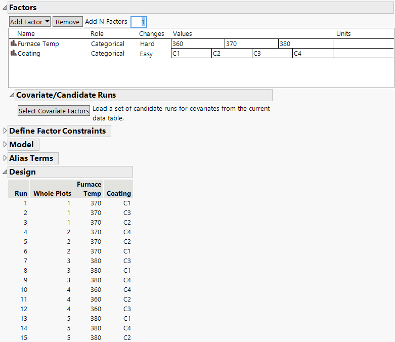
Figure 4.27 Factors and Design Sections for a Split-Plot Design
The Factors section for the corrosion experiment has Changes set to Hard for Furnace Temp and Easy for Coating. The 15-run design consists of five whole plots, within which the settings of Temperature are held constant.
Setup for a Split-Plot Design
In general, several factors can be applied to a processing step where settings are hard-to-change. In the furnace example, you might consider a furnace location factor, as well as temperature. In the Factors section, under the Changes column, you would specify a Changes value of Hard for such factors.
When a custom design involves only easy-to-change and hard-to-change factors, the runs of the hard-to-change factors are grouped using a new factor called Whole Plots. The values of Whole Plots designate blocks of runs with identical settings for the hard-to-change factors. The Model script that is saved to the design table treats Whole Plots as a random effect. See Changes and Design Structure Options.
For an example of creating a split-plot design and analyzing the experimental data, see Split-Plot Experiment.
Split-Split-Plot Designs
A split-split-plot design is used when there are two levels of factors that are hard-to-change. In industry, such designs often occur when batches of material or experimental units from one processing stage pass to a second processing stage. Factors are applied to batches of material at the first stage. Then those batches are divided for second-stage processing, where additional factors are studied. The first stage factors are considered very-hard-to-change, and the second-stage factors are considered hard-to-change. Additional factors can be applied to experimental units after the second processing stage. These factors are considered easy-to-change.
In a split-split-plot design, the batches are considered to be random blocks. Since the batches are divided for second-stage processing, the second-stage factors are nested within the first-stage factors.
Scenario for a Split-Split-Plot Design
Schoen (1999) presents an example of a split-split-plot design that relates to cheese quality. The factors are given in the Cheese Factors.jmp data table found in the Design Experiment folder. The experiment consists of three stages of processing:
• Milk is received from farmers and stored in a large tank.
• Milk from this tank is distributed to smaller tanks used for curd processing.
• The curds from each tank are transported to presses for processing individual cheeses.
The experiment consists of testing:
• Two factors that are applied when the milk is in the large storage tank.
• Five factors that are applied to the smaller curd processing tanks.
• Three factors that are applied to the individual cheeses from a curds processing tank.
Notice that the levels of factors applied to the curd processing tanks (subplots) are nested within the levels of factors applied to the milk storage tank (whole plots).
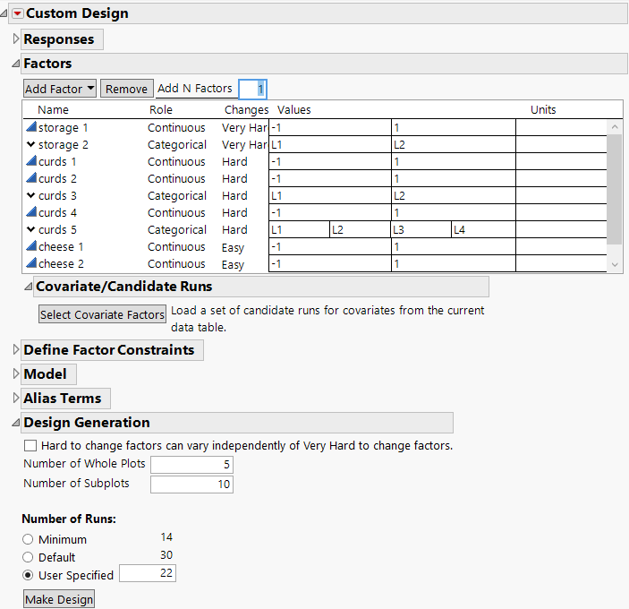
The Factors have Changes set as Very Hard, Hard, or Easy:
• Very Hard for the two storage tank factors.
• Hard for the five curd processing tank factors.
• Easy for the three factors that can be randomly assigned to cheeses.
Figure 4.28 Factors and Design Generation Sections for a Split-Split-Plot Design
The default number of whole plots is 5 and the default number of subplots is 10.The number of runs is set to 22. If only 10 subplots are used the design does not have enough whole plots to estimate the subplot variance. Change the number of subplots to 11 and click Make Design to see a 22-run design.
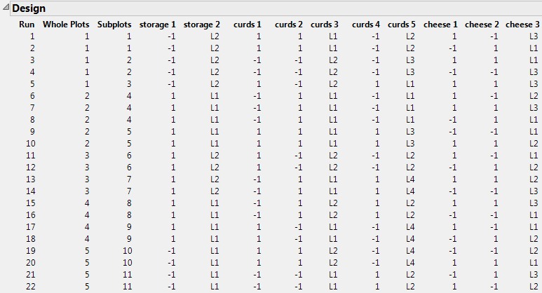
Figure 4.29 Split-Split-Plot Design for Cheese Scenario
The five whole plots correspond to the storage factors; storage 1 and storage 2. The settings of the storage factors are constant within a whole plot. If consecutive whole plots have the same setting for a whole plot factor, the factor should be reset between the plots. For example, you should reset the level for storage 1 between runs 10 and 11 and between runs 14 and 15, and you should reset the level for storage 2 between runs 18 and 19. Resetting the factor between whole plots, even when the specified settings are the same, is required in order to capture whole plot variation.
The 11 subplots correspond to the curds factors. Within a subplot, the settings of the curds factors are constant. Each level of Subplots appears only within one level of Whole Plots, indicating that the levels of Subplots are nested within the levels of Whole Plots.
Levels of the cheese factors vary randomly from run to run.
Setup for a Split-Split-Plot Design
In a split-split-plot design, the Factors section contains factors with Changes set to Very Hard and Hard. The design can also contain factors with Changes set to Easy. Two factors are created:
• A factor called Whole Plots represents the blocks of constant levels of the factors with Changes set to Very Hard.
• A factor called Subplots represents the blocks of constant levels of the factors with Changes set to Hard.
• The factor Subplots reflects the nesting of the levels of the factors with Changes set to Hard within the levels of the factors with Changes set to Very Hard.
• The levels of factors with Changes set to Easy are randomly assigned to units within subplots.
• The factors Whole Plots and Subplots are treated as random effects in the Model script that is saved to the design table.
See the Changes description under Factors Section and Design Structure Options.
Two-Way Split-Plot Designs
A two-way split-plot (also known as strip plot or split block) design consists of two split-plot components. In industry, these designs arise when batches of material or experimental units from one processing stage pass to a second processing stage. But, after the first processing stage, it is possible to divide the batches into sub-batches. The second-stage processing factors are applied randomly to these sub-batches. For a specific second-stage experimental setting, all of the sub-batches assigned to that setting can be processed simultaneously. Additional factors can be applied to experimental units after the second processing stage.
In contrast to a split-split-plot design, the second-stage factors are not nested within the first-stage factors. After the first stage, the batches are subdivided and formed into new batches. Therefore, both the first- and second-stage factors are applied to whole batches.
Although factors at both stages might be equally hard-to-change, to distinguish these factors, JMP denotes the first stage factors as very-hard-to-change, and the second-stage factors as hard-to-change. Additional factors applied to experimental units after the second processing stage are considered easy-to-change.
Scenario for a Two-Way Split-Plot Design
Vivacqua and Bisgaard (2004) describe an experiment to improve the open circuit voltage in battery cells. Two stages of processing are of interest:
• First stage: A continuous assembly process
• Second stage: A curing process with a 5-day cycle time
The engineers want to study six two-level factors:
• Four factors, X1, X2, X3, and X4, that are applied to the assembly process
• Two factors, X5 and X6, that are applied to the curing process
A full factorial design with all factors at two levels would require 26 = 64 runs, and would require a prohibitive 64*5 = 320 days. Also, it is not practical to vary assembly conditions for individual batteries. However, assembly conditions can be changed for large batches, such as batches of 2000 batteries.
Both the first- and second-stage factors are hard-to-change. In a sense, there are two split-plot designs. However, the batches of 2,000 batteries from the first-stage experiment can be divided into four sub-batches of 500 batteries each. These sub-batches can be randomly assigned to the four settings of the two second-stage factors. All of the batches assigned to a given set of curing conditions can be processed simultaneously. In other words, the first- and second-stage factors are crossed.
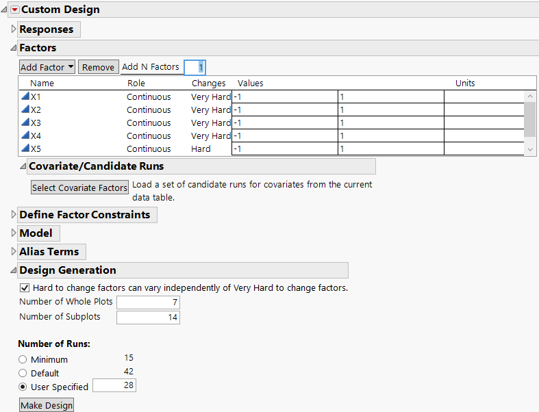
To distinguish between the first- and second-stage factors, you designate the Changes for the first-stage factors as Very Hard, and the Changes for the second-stage factors as Hard (Figure 4.30). Also, under Design Generation, note the following option: Hard to change factors can vary independently of Very Hard to change factors. If this is not checked, the design is treated as a split-split-plot design, with nesting of factors at the two levels. Check this option to create a two-way split-plot design.
Figure 4.30 Factors and Design Generation Sections for a Two-Way Split Plot Design
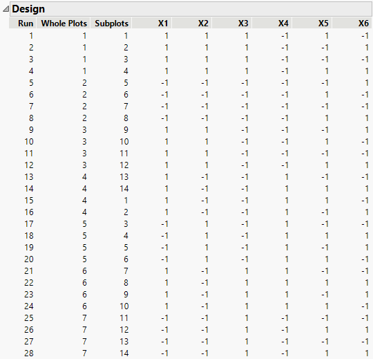
The default number of whole plots is 7; the default number of subplots is 14. Click Make Design to see the 28-run design.
Figure 4.31 Two-Way Split-Plot Design for Battery Cells
The seven whole plots correspond to the first-stage factors, X1, X2, X3, and X4. The settings of these factors are constant within a whole plot. The 14 subplots correspond to the second-stage factors, X5 and X6. For example, the sub-batches for runs 1 and 15 (from different whole plots) are subject to the same subplot treatment, where X5 is set at 1 and X6 at -1.
Setup for a Two-Way Split-Plot Design
A two-way split-plot design requires factors with Changes set to Very Hard and to Hard. As described in Setup for a Split-Split-Plot Design, factors called Whole Plots and Subplots are created. However, in a two-way split-plot design, Subplots does not nest the levels of factors with Changes set to Hard within the levels of factors with Changes set to Very Hard. Both Whole Plots and Subplots are treated as random effects in the Model script that is saved to the design table.
You need to ensure that the factor Subplots is not nested within the factor Whole Plots. Select the option Hard to change factors can vary independently of Very Hard to change factor in the Design Generation section (Figure 4.30). See Changes and Design Structure Options.
For an example of creating a split-plot design and analyzing the experimental data, see Two-Way Split-Plot Experiment.
