Example of Estimating Priors for an Accelerated Life Test Design
In this example, you construct a failure probability optimal ALT test design for a mechanical component. The single acceleration factor is torque, and the normal use stress is 35 Nm (newton meters). You want to estimate the time at which 10% of the units fail at the normal use stress. You construct a failure probability optimal ALT test.
Your test plan has the following characteristics:
• A total of 100 units are available for testing.
• The life distribution is assumed to be Weibull.
• The life-stress relationship is given by the logarithmic transformation.
• You plan to test torque at three stress levels: 50, 75, and 100 Nm.
• You have prior knowledge to predict initial failure times at the test levels. See Obtain Prior Estimates.
• The test runs for 5,000 cycles.
• You will monitor the process for failures on a continuous basis.
Obtain Prior Estimates
To create an accelerated life test design, you must provide prior estimates of the parameters. Here is an approach to obtaining prior estimates:
1. Use your process knowledge to create a table of hypothetical, but likely, failure times at a small number of stress levels.
2. Use the Fit Life by X platform to fit a model and obtain estimates of the model parameters.
3. Use these estimates as your prior values for creating a design using the ALT Design platform.
Follow the approach outlined above with a data table containing estimates of the number of failure cycles for a balanced design.
1. Select Help > Sample Data Folder and open Design Experiment/Torque Prior.jmp.
2. Select Analyze > Reliability and Survival > Fit Life by X.
3. Select Cycles and click Y, Time to Event.
4. Select Torque and click X.
5. From the Relationship list, select Log.
6. Enter 35 for the Use Condition. Recall that 35 Nm is the normal use condition.
7. From the Distribution list, select Weibull.
Figure 23.8 Fit Life by X Launch Window
8. Click OK.
9. Scroll down to the Weibull Results section and open the Correlation Matrix section.
Figure 23.9 Fit Life by X Model for Prior Data
The model for the mean is given in the Estimates section. The Estimate column contains the parameter estimates for the intercept (β0), the linear coefficient (β1), and the scale (σ). The standard errors column contains the standard errors for the estimates. The estimated correlations for the parameter estimates are given in the Correlation Matrix section. Use these parameter estimates, standard errors, and correlations as your prior values to construct your ALT design.
Enter Basic ALT Design Specifications
Use the estimated priors to create the accelerated life test design.
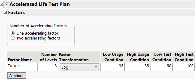
1. Select DOE > Special Purpose > Accelerated Life Test Design.
Notice that One accelerating factor is selected by default.
2. Under Factor Name, click X1 and type Torque.
Notice that the Number of Levels is set to 3 by default.
3. Select Log under Factor Transformation.
4. Enter 35 for both the Low Usage Condition and the High Usage Condition.
Setting both the low and high usage conditions to 35 indicates that 35 is the normal usage condition.
5. Enter 50 for the Low Test Condition and 100 for the High Test Condition.
Figure 23.10 Completed ALT Specification Window
6. Click Continue.
Enter Prior Specifications
1. Click the Accelerated Life Test Plan red triangle and select ALT Optimality Criterion > Make Failure Probability Optimal.
2. Ensure that Weibull is selected as the Distribution Choice.
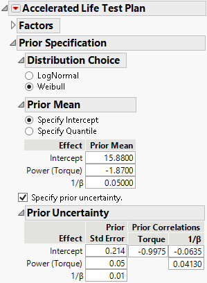
1. Under Prior Mean, select Specify Intercept and enter the prior acceleration model parameter estimates that you obtained using the Fit Life by X platform with your hypothetical data:
– Enter 15.88 for Intercept.
– Enter -1.87 for Power (Torque).
– Enter 0.05 for 1/β (scale parameter for a Weibull model).
2. Select Specify prior uncertainty.
3. Enter the estimated standard errors and correlations from the prior acceleration model. Figure 23.11 shows the completed Prior Uncertainty section:
Figure 23.11 Completed Prior Specifications
4. Click Continue.
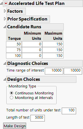
Notice the Torque Level Values are set to 50, 75, and 100.
Note: JMP sets the values of the levels evenly spaced between the low and high test conditions. You can change the levels.
You plan to conduct the test over 5,000 cycles. You are interested in predictions for as many as 10,000 cycles.
5. In the Diagnostic Choices section, enter 10,000 for both boxes for Time range of interest.
6. In the Design Choices section, ensure that Continuous Monitoring is selected as the Monitoring Type.
7. Enter 100 for the Total number of units under test.
8. Enter 5,000 for Length of test.
Figure 23.12 Completed Diagnostic and Design Choices
Make the Design
Continue the ALT example by generating the design.
1. Click Make Design.
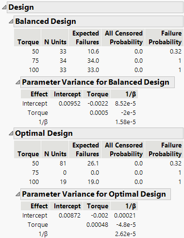
Figure 23.13 ALT Designs
The Design report provides a balanced and an optimal design with parameter variance covariance matrices for the parameters. You can compare the parameter variance estimates of the two designs and see that the biggest difference is in the estimation of 1/β. The primary difference between the designs is that the optimal design requires only two Torque settings.
The optimal design is computed based on the levels of the test runs, the total number of units to be tested, and the prior information that you specified. The optimal design consists of testing the specified number of units at each torque level:
– 82 units at 50 Nm
– 0 units at 75 Nm
– 18 units at 100 Nm
Design Diagnostics
The Design Diagnostics report contains optimality criteria, a distribution profiler, and an R Precision Factor profiler for the optimal design. Note that the R precision factor profiler shows very little variation across all three inputs. This indicates that the design is stable with the specified 100 samples.
Run Simulations
Evaluate the proposed ALT design with the simulator. Use the simulator to simulate the results of your test plan based on the assumptions used to build the design. This is a way to evaluate if the test plan is sufficient before running the test plan.
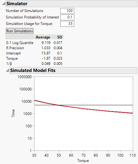
1. Enter 100 for the Number of Simulations.
2. Enter 0.1 for the Simulation Probability of Interest.
3. Enter 35 for the Simulation Usage for Torque.
4. Click Run Simulations to run 100 simulations of the experiment. This is to check to see whether the 100 units that you plan to test are sufficient given your prior assumptions for the design.
Figure 23.14 Simulation Results
The simulated model fits shows that the 100 simulations of the model are all similar as they all fall close to the average shown by the red curve. The Y axis is on a log scale.
5. Use the magnifier tool to view the fits around the 35 normal usage condition. If helpful, change the Y-axis scale from log to linear. Double-click the Y axis and select Linear from the Type menu and click OK.
You expect variability in your estimated of the normal usage condition. The simulation helps you evaluate if your ALT plan is acceptable. If there is too much variability, you might need to increase the number of units on test or adjust the test conditions.
Save Design
Complete the example ALT design by making a test plan and saving it to a data table.
1. Click Make Test Plan to save the design to a data table. This table is a summary of the design.
2. Click Make Table to save the design to a data table. This table has 100 rows, one for each test run.
