Optimality Criterion for Accelerated Life Tests
Consider an accelerated life test (ALT) to be conducted across at most two acceleration factors x1 and x2 with J1 and J2 levels, respectively. The goal of test planning is to determine the number of samples to allocate to each combination of the factor levels.
The computation of the optimality criterion depends on the overall Fisher information matrix from the individual level-specific information matrices

as well as the inclusion of prior uncertainty S where appropriate.
D-optimality
The D-optimal design Dd is the design that minimizes the following expression across all possible values of njj

where |·| is the determinant operation and π(θ) is the prior distribution over the parameters. This distribution is usually a multivariate normal distribution. The log of the determinant is used for numerical stability.
Quantile Optimality
The quantile optimal design Dq is the design that minimizes the expression:

where the vector c depends on the use condition.
For the single use condition

where zp is the pth quantile of the failure distribution.
For the range of use condition let

where G(·) is the antiderivative of g(·), xiUh is the highest use level considered for the ith factor, xiUl is the lowest use level considered for the same factor. Then

where zp is the pth quantile of the failure distribution.
Failure Probability Optimality
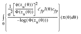
The failure probability optimal design Df is the design that minimizes the expression:

where zU(θ) is the standardized log-time at use conditions as defined in Quantile Optimality. cfp is similar to c as defined in Quantile Optimality except that the last entry is zU(θ). The quantity in the numerator is based on the asymptotic variance of logΦ(zU(θ)), where the log-transformation is used for numerical stability. The asymptotic variance is then standardized in terms of the original logΦ(zU(θ)) for consistency and smaller is better. For a range of use conditions, the integral is taken inside of logΦ(·) rather than over the asymptotic variance for ease of computation. It is still appropriate as an optimality metric by the property that the variance of a sum bounds the sum of variances and both the logarithmic function and cdf are monotone functions. As such, minimizing the above expression minimizes the true asymptotic variance of the failure probability by bounding it from above.