Simulate Responses
Use simulated responses for exploration of a design prior to data collection or in a classroom setting. When simulate responses is selected and you click Make Table to create your design table, the Simulate Responses option performs the following actions:
• Adds random response values to the response column(s) in your design table.
• Adds a new a column for each response containing a simulation formula to the design table.
• Opens a model window that enables you to specify the simulation. When you click Apply in the Model window, each column containing a simulation model formula is updated.
Simulate Responses
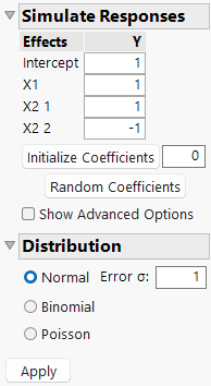
The initial simulation sets the model coefficients at 1 and adds error simulated from a Normal distribution with standard deviation equal to 1. If you have set Anticipated Coefficients as part of Power Analysis under Design Evaluation in the DOE window, then the default values in the Simulate Responses section are the values that you specified as Anticipated Coefficients and Anticipated RMSE (Error Std) in the Power Analysis section. If it is not possible to fit the model specified in the data table’s Model script, the intercept and coefficients have default values of 0.
The linear model used to simulate the response values is defined by the following linear function:
L(x, β) = x‘β + ε
where:
– The vector x consists of the terms that define the effects listed under Effects.
– The vector β is the vector of model coefficients that you specify under Y.
– The error term ε is simulated from the specified distribution.
Figure 4.27 shows the Model window for a design with one continuous factor (X1) and one three-level categorical factor (X2). Notice that X2 is represented by two model terms.
Note: For definitive screening designs, the Model window contains a Factors section to enable you to add terms to the simulated model.
Figure 4.27 Simulate Responses Model Window
To specify specific model effects, enter values for the coefficients for each model term and click Apply. Use the Initialize Coefficients button to set all coefficients to the value that you specify in the text box. Use the Random Coefficients button to randomly set coefficients. Click the Apply button to update the simulation.
Show Advanced Options
Shows or hides advanced simulation options. For more information about effect sparsity, effect hierarchy, and model heredity see “Principles and Guidelines for Experimental Design”.
Set Random Seed
Enables you to specify a random seed used in the generation of the random coefficients.
Enforce Effect Sparsity
Enables you to specify the proportion of nonzero main effects (MEs), two-factor interactions (2FIs), and quadratic (Quads) coefficients for the model simulation. Specify a proportion between 0 and 1 for each type of model term.
Enforce Effect Hierarchy
Enables you to set the size of the two-factor interactions (2FIs), and quadratic (Quads) coefficients relative to the main effect coefficients. Specify a relative size between 0 and 1.
Enforce Model Heredity
Enforces model heredity if selected. This means that models include lower-order components of higher-order effects.
Note: After setting advanced options, click the Random Coefficients button to update the coefficients. Then click the Apply button to update the simulated responses.
Distribution
Choose from one of the available distributions in the Simulate Responses window:
Normal
Adds one or more random error terms to the linear model defined by the design and the specified coefficients. The errors are simulated from a normal distribution. Use the normal distribution for continuous responses. Enter a value for Error σ, the standard deviation of the normal error distribution. If you have designated factors to have Changes of Hard in the Factors section, you can enter a value for Whole Plots σ, the whole plot error. If you have designated factors to have Changes of Hard and Very Hard, you can enter values for both the subplot and whole plot errors. When you click Apply, the simulation formula is updated in the column <Y> Simulated.
Note: The Normal Error σ is the anticipated root mean square error.
Binomial
Simulates values from a binomial distribution. Use the binomial distribution for dichotomous responses. Enter a value for N, the number of trials. Random integer values are generated according to a binomial distribution based on N trials with probability of success 1/(1 + exp(-L(x, β)). When you click Apply, the simulation formula is updated in the column <Y> Simulated. A column called N Trials that contains the value N is also added to the data table.
Poisson
Simulates random integer values according to a Poisson distribution with parameter exp((L(x, β)). Use the Poisson distribution for count responses. When you click Apply, the simulation formula is updated in the column <Y> Simulated.
Note: You can set a preference to simulate responses every time you click Make Table. To do so, select File > Preferences > Platforms > DOE. Select Simulate Responses.
