Tip: If you find that the report window is too long, select Tabbed Report from the red triangle menu.
|
•
|
The time period when it is not known if the units in the row are functioning is indicated with a dashed line.
|
In the Fan.jmp sample data table there is a single Time column indicating failure time. When the failure time is unknown, the value Censored is recorded in the Censor column. All censored units are assumed to be right-censored. Event Plot for Right-Censored Data shows the Event Plot for this data.
Note: To construct the plot in Event Plot for Right-Censored Data, select Help > Sample Data Library and open Reliability/Fan.jmp. Select Run Script from the red triangle menu for the script Life Distribution - Exponential. Click the Event Plot disclosure icon.
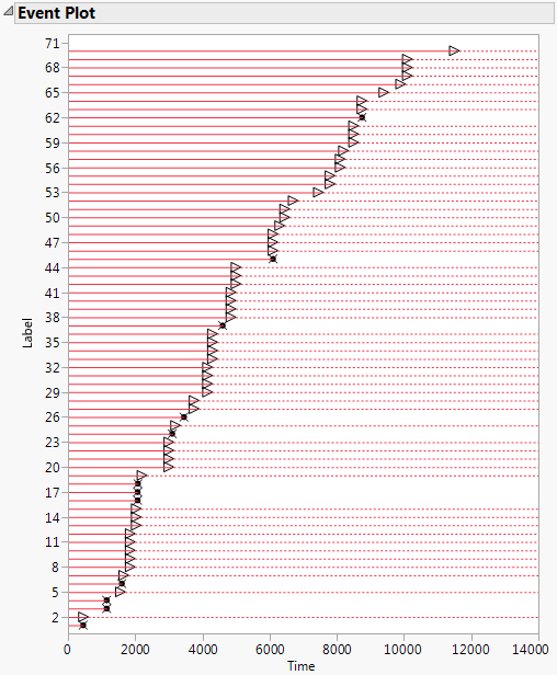
The unit in row 3 failed at Time 1150. Its lifetime is represented by a solid horizontal line that ends at Time 1150. The failure time is marked with an “x”.
The unit in row 5 is right censored. It was last know to be functioning at Time 1560. The time period during which the unit is known to be functioning is represented by a solid horizontal line that ends at Time 1560. At Time 1560, a right arrow is plotted. The line continues as a dashed line, indicating that the failure time is unknown, but greater than 1560.
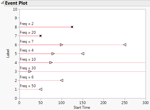
In the Censor Labels.jmp sample data table, there are two columns, Start Time and End Time. Start Time indicates when units in a row were last known to be functioning. End Time indicates when units in that row were first known to have failed.
|
•
|
Units in rows 1 and 2 are left censored. They were known to fail before the time in the End Time column, but their exact failure times are unknown.
|
|
•
|
Units in rows 3 and 4 are right censored. They were known to be last functioning at the time in the Start Time column, but their failure times are unknown.
|
|
•
|
|
•
|
Units in rows 7 and 8 are not censored. Their failure times are given by the values in the Start Time and End Time columns, which are identical.
|
Event Plot for Mixed-Censored Data shows the Event Plot for this data.
Note: To construct the plot in Event Plot for Mixed-Censored Data, select Help > Sample Data Library and open Censor Labels.jmp. Select Run Script from the red triangle menu for the script Life Distribution. Click the Event Plot disclosure icon.
|
•
|
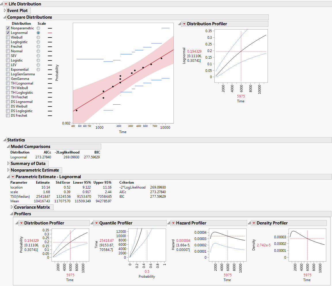
Select a distribution for the response. Different distributions appear based on characteristics of the data. For details about which distributions are available, see Available Parametric Distributions.
|
•
|
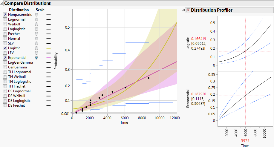
Compare Distributions Report and Distribution Profiler shows an example of the Compare Distributions report. The Logistic (yellow) and Exponential (magenta) distributions are shown. The plot is scaled using the Exponential distribution.
Note: Distributions for the Competing Cause report are covered in Available Distributions for Competing Cause Compare Distributions Reports.
The available distributions are listed and described in detail in Parametric Distributions. There are four major groupings of parametric distributions:
You can restrict which distributions are available by default by deselecting the ones that you do not want to appear. Select File > Preferences > Platforms > Life Distribution. The distributions listed include the Threshold, Defective Subpopulation, Zero-Inflated, LogGenGamma, and GenGamma distributions. By default, all of the distributions are checked and available.
|
•
|
|
•
|
|
•
|
|
•
|
|
•
|
|
•
|
|
•
|
In the case of zero-failure data, none of the above distributions are available by default. However, you can uncheck the preference called Weibayes Only for Zero Failure Data. This enables you to obtain Bayesian fits for those distributions where the Bayesian Estimate option is available. See Weibayes Only for Zero Failure Data.
|
•
|
|
•
|
|
•
|
|
•
|
|
•
|
|
•
|
A list of distributions that are available as priors for hyperparameters of these distributions is given in Prior Distributions for Bayesian Estimation.
|
•
|
Parametric Estimate - <Distribution Name> (one report appears for each distribution that you select in the Compare Distributions report)
|
Initially, the rows are sorted by AICc. To change the statistic used to sort the report, select Comparison Criterion from the Life Distribution red triangle menu. See Life Distribution Report Options for details about this option.
See Nonparametric Fit for more information about nonparametric estimates.
Opens a report where you can specify the value of parameters. Enter your fixed parameter values, select the appropriate check box, and then click Update. JMP re-estimates the other parameters, covariances, and profilers based on the new parameters, and shows them in the Fix Parameter report. For an example in a competing cause situation, see Specify a Fixed Parameter Model as a Distribution for a Cause.
For the Weibull distribution, the Fix Parameter option lets you select the Weibayes method. For an example, see Weibayes Estimates. The Weibayes option is not available for interval-censored data.
Performs Bayesian estimation of parameters for certain distributions based on three methods of specifying prior distributions (Location and Scale Priors, Quantile and Parameter Priors, and Failure Probability Priors). See Bayesian Estimation - <Distribution Name>. This option is available only for the following distributions: Lognormal, Weibull, Loglogistic, Fréchet, Normal, SEV, Logistic, LEV.
Provides calculators that enable you to predict failure probabilities, survival probabilities, and quantiles for specific time and failure probability values. Each calculated quantity includes confidence intervals, which can be two-sided or one-sided (in either direction). Two reports appear: Estimate Probability and Estimate Quantile. See Custom Estimation.
Provides a calculator that enables you to estimate the mean remaining life of a unit. In the Mean Remaining Life Calculator, enter a Time and press Enter to see the estimate. Click the plus sign to enter additional times. This calculator is available for the following distributions: Lognormal, Weibull, Loglogistic, Fréchet, Normal, SEV, Logistic, LEV, and Exponential.
From the Parametric Estimate - <Distribution Name> report outline, select Bayesian Estimates. This opens an outline called Bayesian Estimation - <Distribution Name>. The initial report is a control panel where you can specify the parameters for the priors and control aspects of the simulation.
|
•
|
Enables you to specify hyperparameters for prior distributions on generic parameters (location and scale parameters). Select the Prior Distribution red triangle menu to select a distribution for each parameter. You can enter new values for the hyperparameters of the priors. The initial values that are provided are estimates consistent with the MLEs. For details, see Prior Distributions for Bayesian Estimation.
Enables you to specify prior information about a quantile and the scale parameter (or Weibull beta if the parametric fit is Weibull). The quantile is defined by the value next to Probability. The default Probability value is 0.10, but you can specify a value that corresponds to the quantile of interest. Specify information about the prior information in terms of Lower and Upper 99% limits on the range of each prior distribution. See Meeker and Escobar, 1998. The initial values that are provided are estimates consistent with the MLEs. For details, see Prior Distributions for Bayesian Estimation.
The values shown in the Distribution Profiler, at a given time t, are calculated as follows:
|
‒
|
|
‒
|
The plot and confidence limits shown in the Quantile Profiler are obtained in a similar fashion. For a given Probability value p, the quantiles corresponding to p are calculated from the distributions associated with the posterior parameter values.
In a zero-failure situation, no units fail. All observations are right censored. If you have zero-failure data, it is possible to conduct either Bayesian estimation or Weibayes inference. See Weibayes Report.
Note: By default, zero-failure data is analyzed using the Weibayes method. If you want to conduct a broader Bayesian analysis on zero-failure data, uncheck the preference Weibayes Only for Zero Failure Data, located under File > Preferences > Platforms > Life Distribution.
The Custom Estimation option produces two reports: Estimate Probability and Estimate Quantile. The Estimate Probability report contains a calculator that enables you to predict failure and survival probabilities for specific time values. The Estimate Quantile report contains a calculator that enables you to predict quantiles for specific failure probability values. Both Wald-based and likelihood-based confidence intervals appear for each estimated quantity. The confidence level for these intervals is determined by the Change Confidence Level option in the Life Distribution red triangle menu.
In the Estimate Probability calculator, enter a value for Time. Press Enter to see the estimates of failure probabilities, survival probabilities, and corresponding confidence intervals. To calculate multiple probability estimates, click the plus sign, enter another Time value in the box, and press Enter. Click the minus sign to remove the last entry.
In the Estimate Quantile report, enter a value for Failure Probability. Press Enter to see the quantile estimates and corresponding confidence intervals. To calculate multiple quantile estimates, click the plus sign, enter another Failure Probability value in the box, and press Enter. Click the minus sign to remove the last entry.