|
1.
|
Select DOE > Space Filling Design.
|
|
3.
|
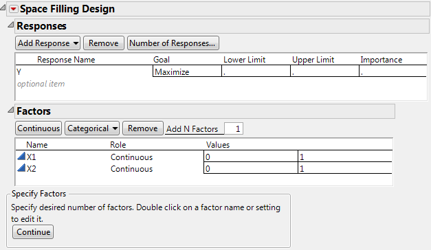
Alter the factor level values, if necessary. For example, Space-Filling Dialog for Two Factors shows the two existing factors, X1 and X2, with values that range from 0 to 1 (instead of the default –1 to 1).
|
|
4.
|
Click Continue.
|
|
5.
|
In the design specification dialog, specify a sample size (Number of Runs). Space-Filling Design Dialog shows a sample size of eight.
|
|
6.
|
Click Sphere Packing.
|
JMP creates the design and displays the design runs and the design diagnostics. Sphere-Packing Design Diagnostics shows the Design Diagnostics panel open with 0.518 as the Minimum Distance. Your results might differ slightly from the ones below, but the minimum distance is the same.
|
7.
|
Click Make Table. Use this table to complete the visualization example, described next.
|
|
•
|
Add circles using the minimum distance from the diagnostic report shown in Sphere-Packing Design Diagnostics as the radius for the circles.
|
|
1.
|
Select Graph > Overlay Plot.
|
|
2.
|
|
3.
|
Adjust the frame size so that the frame is square by right-clicking the plot and selecting Size/Scale > Size to Isometric.
|
|
4.
|
Right-click the plot and select Customize. When the Customize panel appears, click the plus sign to see a text edit area and enter the following script:
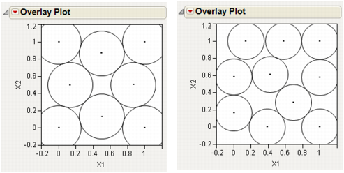
For Each Row(Circle({:X1, :X2}, 0.518/2)) where 0.518 is the minimum distance number that you noted in the Design Diagnostics panel. This script draws a circle centered at each design point with radius 0.259 (half the diameter, 0.518), as shown on the left in Sphere-Packing Example with Eight Runs (left) and 10 Runs (right). This plot shows the efficient way JMP packs the design points. |
Remember to change 0.518 in the graphics script to the minimum distance produced by 10 runs. When the plot appears, again set the frame size and create a graphics script using the minimum distance from the diagnostic report as the diameter for the circle. You should see a graph similar to the one on the right in Sphere-Packing Example with Eight Runs (left) and 10 Runs (right). Note the irregular nature of the sphere packing. In fact, you can repeat the process a third time to get a slightly different picture because the arrangement is dependent on the random starting point.