The Contrasts outline lists model effects, a contrast value for each effect, Lenth t-ratios (calculated as the contrast value divided by the Lenth PSE (pseudo-standard error), individual and simultaneous p-values, and aliases if there are any. Effects are entered into the analysis following a hierarchical ordering. See Order of Effect Entry for details. Effects with Individual p-Value less than 0.10 are highlighted.
|
Shows the Lenth t-ratios with blue vertical lines indicating a value that is significant at the 0.10 level.
|
|
|
Lenth’s t-ratio, calculated as
|
|
|
Analogous to the standard p-values for a linear model. Small values of this value indicate a significant effect. Refer to Lenth’s Pseudo-Standard Error for details.
Do not expect the p-values to be exactly the same if the analysis is re-run. The Monte Carlo method should give similar, but not identical, values if the same analysis is repeated.
|
|
|
Similar to the individual p-value, but multiple-comparison adjusted.
|
|
The Make Model button beneath the Half Normal Plot creates a Fit Model dialog that includes all the highlighted effects.
|
1.
|
Open the Plackett-Burman.jmp sample data table, found in Design Experiment folder.
|
|
2.
|
|
3.
|
Click OK.
|
|
4.
|
Click the Make Model Button beneath the Half Normal Plot.
|
Note that the Catalyst*Stir Rate interaction is highlighted, but the Stir Rate main effect is not. In accordance with the principle of Effect Heredity, add the Stir Rate main effect to the model. See Effect Heredity in Starting Out with DOE.
|
5.
|
|
6.
|
Click Run.
|
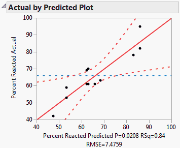
The Whole Model actual-by-predicted plot, shown in An Actual-by-Predicted Plot, appears at the top of the Fit Model report. You see at a glance that this model fits well. The blue line falls outside the bounds of the 95% confidence curves (red-dotted lines), which tells you the model is significant. The model p-value (p = 0.0208), R2, and RMSE appear below the plot. The RMSE is an estimate of the standard deviation, assuming that the unestimated effects are negligible.
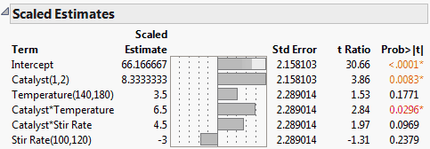
To see a scaled estimates report, use Effect Screening > Scaled Estimates found in the red triangle menu on the Response Percent Reacted title bar. When there are quadratic or polynomial effects, the coefficients and the tests for them are more meaningful if effects are scaled and coded. The Scaled Estimates report includes a bar chart of the individual effects embedded in a table of parameter estimates. The last column of the table has the p-values for each effect.
The Fit Model report has outline nodes for the Catalyst and Temperature effects. To run a power analysis for an effect, click the red triangle icon on its title bar and select Power Analysis.
This example shows a power analysis for the Catalyst variable, using default value for α (0.05), the root mean square error and parameter estimate for Catalyst, for a sample size of 12. The resulting power is 0.8926, which means that in similar experiments, you can expect an 89% chance of detecting a significant effect for Catalyst.
Refer to the Fitting Linear Models book for details.


