Degrees of Freedom
What are degrees of freedom?
Degrees of freedom tell you how many independent pieces of information you have. Any parameter to be estimated has associated degrees of freedom. Degrees of freedom are important in estimating variability, testing hypotheses, or fitting models.
What is an example of degrees of freedom?
Suppose someone has three observations and tells you their average value, would you know what the three values are? No! But if they tell you two of the three observations and the average, then you can figure out the last observation.

The first two numbers can be chosen freely, but the third is determined by the given average. The number of terms that can be chosen freely is the degrees of freedom. In this example, there are three observations, and one parameter is being estimated (the mean). The number of degrees of freedom is 3 – 1 = 2. Similarly, if there were 100 values and you knew the average, there would be 99 degrees of freedom.
Why do degrees of freedom matter?
Reference distributions
Degrees of freedom affect the shape of many reference distributions, such as the t, chi-square ($\chi^2$), and F distributions. You can see different t, $\chi^2$, and F density functions in the figures below. In the first panel, the lowest t density function has just 1 df. As the degrees of freedom increase, the tails of the t density become thinner and the peak becomes taller. The t approaches the normal distribution as degrees of freedom increase. The second panel shows various density functions. As degrees of freedom increase, the $\chi^2$ also approaches the normal distribution. Various F densities are shown in the third panel. The F distribution has two parameters (the numerator degrees of freedom and the denominator degrees of freedom), because it arises from a ratio of variances of normally distributed data.


Critical values and p-values
Degrees of freedom also help determine the correct critical values and p-values in hypothesis tests.
The figure below shows the results of three hypothesis tests, all with the same calculated test statistic. The value of the test statistic is 3.4 for all three tests and is represented with a red line. The critical value of the reference distribution depends on the degrees of freedom and significance level (here, $\alpha$ = 0.05) and is represented by a blue line. Different hypothesis tests with different sample sizes have different critical values. Whether that hypothesis test is deemed significant or not depends on the reference distribution.
The first graph represents a one-samplet-test with 12 df. It is significant because the red line at 3.4 is much larger than the blue line at the critical value of 1.78. The middle graph represents a chi-square test of independence for a contingency table with 3 df. It is not significant because the red line at 3.4 is much smaller than the critical value of 7.81. The final graph represents an F-test in an ANOVA table with (10, 8) df. It is weakly significant because the red line at 3.4 is very close to the critical value of 3.34.

Model complexity
Degrees of freedom help describe model complexity in linear models. When you fit a linear model, you can then calculate an ANOVA table containing a row for each parameter estimated. There is one degree of freedom used to estimate the mean or intercept. This term is not typically included in the ANOVA table. Instead, the corrected total degrees of freedom are listed as $n – 1$. Degrees of freedom account for information used up when estimating parameters from data. The more parameters in your model, the more degrees of freedom your model uses.
In simple linear regression, 1 df is used to estimate the intercept and 1 df is used to estimate the slope. There are $n – 2$ df for the error term. In the figure below, soil pH has been measured in 20 fields that grow cotton crops. The researcher has also measured a quality index for the crop in each field and is interested in understanding how pH affects the quality index.

The ANOVA table shown below has $1$ df for the model which has one slope to estimate, $n – 1 = 20 – 1 = 19$ df for the corrected total (the 1 is for the intercept), and $n – 2 = 20 – 2 = 18$ df for the error term.
| Source | DF | Sum of squares | Mean square | F | p |
| Model | 1 | 213.94183 | 213.942 | 33.0716 | <0.0001 |
| Error | 18 | 116.44305 | 6.469 | ||
| C. total | 19 | 330.38488 |
In one-way ANOVA, $1$ df is used to estimate the overall mean. Because the overall mean has been estimated, you only need to know $k – 1$ group means. Therefore, for $k$ groups, $k – 1$ df are used to estimate the group means, and there are $n – k$ df for the error term. In the figure below, three additives are used in a new insulator. The change in temperature from a set value is recorded; a lower value means the additive forms a better insulator. There are 10 measurements for each additive.

The ANOVA table below shows $3 – 1 = 2$ df for Additive. There are $30$ measurements total, so there are $30 – 1 = 29$ df for the corrected total, which leaves $29 – 2 = 27 df$ for the error term.
| Source | DF | Sum of squares | Mean square | F | p |
| Additive | 2 | 34.41052 | 17.2053 | 4.6275 | 0.0187 |
| Error | 27 | 100.38696 | 3.7180 | ||
| C. total | 29 | 134.79748 |
In linear models, each categorical factor uses $k – 1$ df for $k$ groups, each continuous factor uses 1 df for one slope. The df for an interaction term is the product of the df for the factors in the interaction. For example, if factor A is a categorical factor with three levels, it has 2 df. If factor B is a continuous factor, it has 1 df. The A´B interaction term has 2 x 1 = 2 df. The df for the error term is $n – 1$ minus the sum of the df of all the terms in the model.
Suppose a researcher is interested in the effect of two diluents and four buffers on the pH of a solution. She designs a full factorial experiment with replication and makes 16 runs. A graph of the data is shown in the figure below.
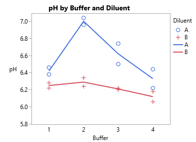
Diluent has two levels and $2 – 1 = 1$ df. Buffer has four levels and $4 – 1 = 3$ df. The Diluent´Buffer interaction effect has $(2 – 1) ´ (4 – 1) = 1 ´ 3 = 3$ df. The corrected total sum of squares has $n – 1 = 16 – 1 = 15$ df. The error term has $15 – 1 – 3 – 3 = 8$ df. The ANOVA table is in the figure below.
| Source | DF | Sum of squares | Mean square | F | p |
| Diluent | 1 | 0.5625 | 0.5625 | 61.1413 | e. 15e-5 |
| Buffer | 3 | 0.38 | 0.1267 | 13.7681 | 0.00159 |
| DiluentxBuffer | 3 | 0.1827 | 0.0609 | 6.6196 | 0.01468 |
| Error | 8 | 0.0736 | 0.0092 | ||
| C. total | 15 | 1.1988 |