k-Nearest Neighbors (KNN) Model

How do you build a KNN model?

Let’s look at a simple example to illustrate how KNN models work. Suppose you have the following data, found in the table below. There is one input, X, and one output, Y.

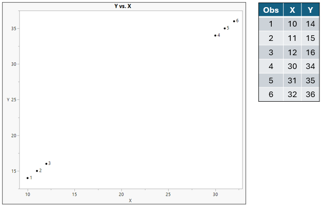
Let’s start with the model for k = 1. We will go through the observations, one at a time, determine the nearest neighbor, then use that observation as the prediction.

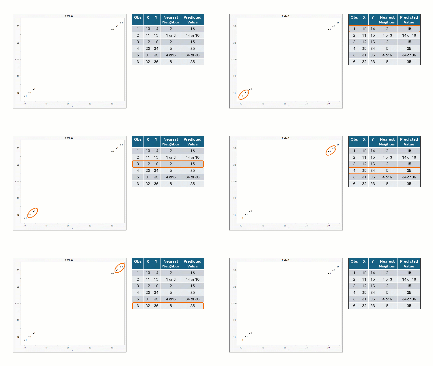
When k = 1, the nearest neighbor for each point is found using a scaled Euclidean distance. The predicted value for each observation is the value of the nearest neighbor. In the event of a tie, one of the nearest neighbors is chosen at random.

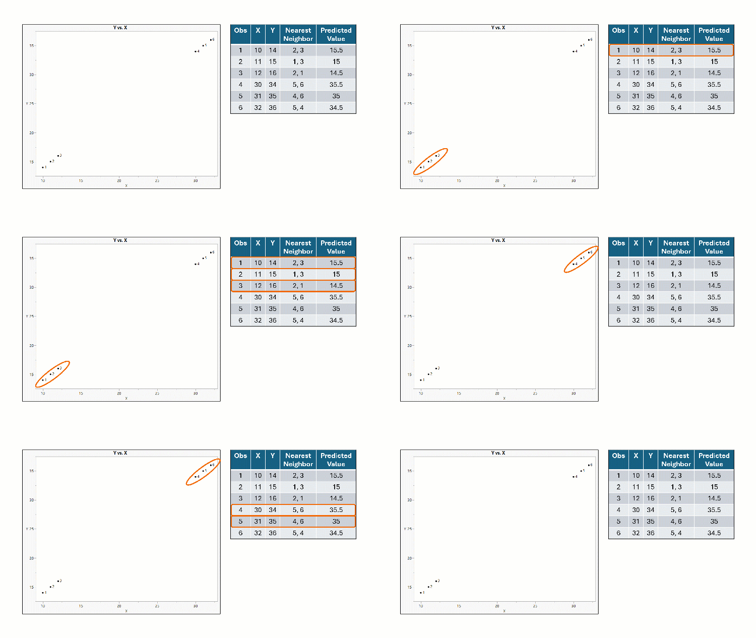
When k = 2, the two closest neighbors to an observation are used to create the prediction. For a continuous response, the prediction is the average of the nearest neighbors. For a categorical response, the prediction is the most frequent level for all neighbors. This approach can be generalized to larger values of k.

To determine the best value of k, evaluate models from k = 1 up to a user-specified value, and choose the value that performs best on a validation set.

What are the advantages and disadvantages of KNN models?

Advantages

• KNN approach can model continuous or categorical responses, such as the yield of a manufacturing lot (continuous) or the pass/fail status of the lot (two-level categorical).
• KNN easily handles multinomial responses, such as a three-level lot status: pass, fail, or requires additional testing.

Disadvantages

• The prediction formula can be hard to interpret because predictions are based on the values of nearby observations rather than a simple mathematical formula.
• KNN suffers from the curse of dimensionality – if the data are sparse in high dimensions, the method can fail to produce good predictions.
• For a categorical response, the model predicts only the category, not the probability of being in that category. Other methods, such as neural networks and decision trees, can provide both the predicted category and the probability for each possible category.
• The method might be sensitive to outliers because unusual observations that are selected as nearest neighbors can greatly influence predictions.

Example of a KNN model

Let’s fit a KNN model on the Recovery data we introduced in our overview of predictive modeling. We’ll look at the continuous response Percent Recovered.

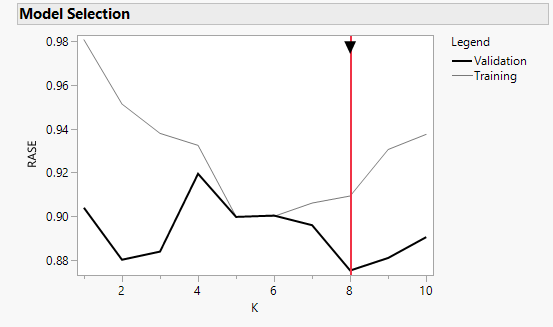
The picture above shows the model performance as a function of k for k = 1 to 10. The Y axis is the square root of the average squared error (RASE), and smaller is better. The minimum value of RASE on the validation set occurs at k = 8. You compare models (for example, different values of k) using the validation set to help avoid overfitting and then choose the value of k that works best on new data.

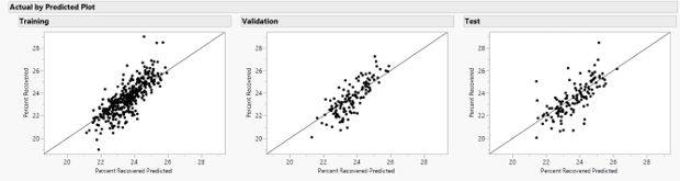
The plot of actual values by predicted values for the KNN model with k = 8 shows slight model bias on both the training and validation sets. On average, high values are being predicted lower, and lower values are being predicted higher than they actually are.