Findings Box Plots
This report displays the box plots by treatment group representing the change from baseline in measurements for each test for specified findings domain across various times or points in the study. Times can be specified using a list of bracketed times or, alternatively, a number of times can be set to create times that span across the entire study.
If the variable xxBLCHG (where xx is substituted with the chosen domain 2 letter code) exists, this variable is used in plotting change from baseline. Otherwise, a measurement is determined to be a baseline measurement by the ABLFL or xxBLFL variable where xx is substituted with the 2-letter code for the chosen domain for analysis. If this variable does not exist, baseline is calculated from measurements taken on or before day 1 of the study. A time can be specified to determine baseline measurements.
Note: JMP Clinical uses a special protocol for data including non-unique Findings test names. Refer to How does JMP Clinical handle non-unique Findings test names? for more information.
Methodology
Counts of subjects with findings results are tabulated for each visit. Mean, median, standard deviation, minimum and maximum values are computed for selected findings test for each visit.
Usage and Interpretation
The Findings Box Plots report supports exploratory review of continuous findings data across visits. The report can be used to evaluate distributions, identify outliers, compare treatment groups, assess changes from baseline, and identify subjects who may warrant additional investigation. Visual patterns and summary statistics can help identify trends, outliers, and potential safety signals, but differences observed are not based on formal statistical testing. The following examples illustrate common review scenarios.
Note: Click on the figures below to enlarge.
Example 1: Mean Change from Baseline in BUN Over Time by Treatment
In this example, report options were set as shown in the following table:
| Option Type | Option | Setting | |
|---|---|---|---|
| Display | Laboratory Test Results | Blood Urea Nitrogen (mMol/L) | 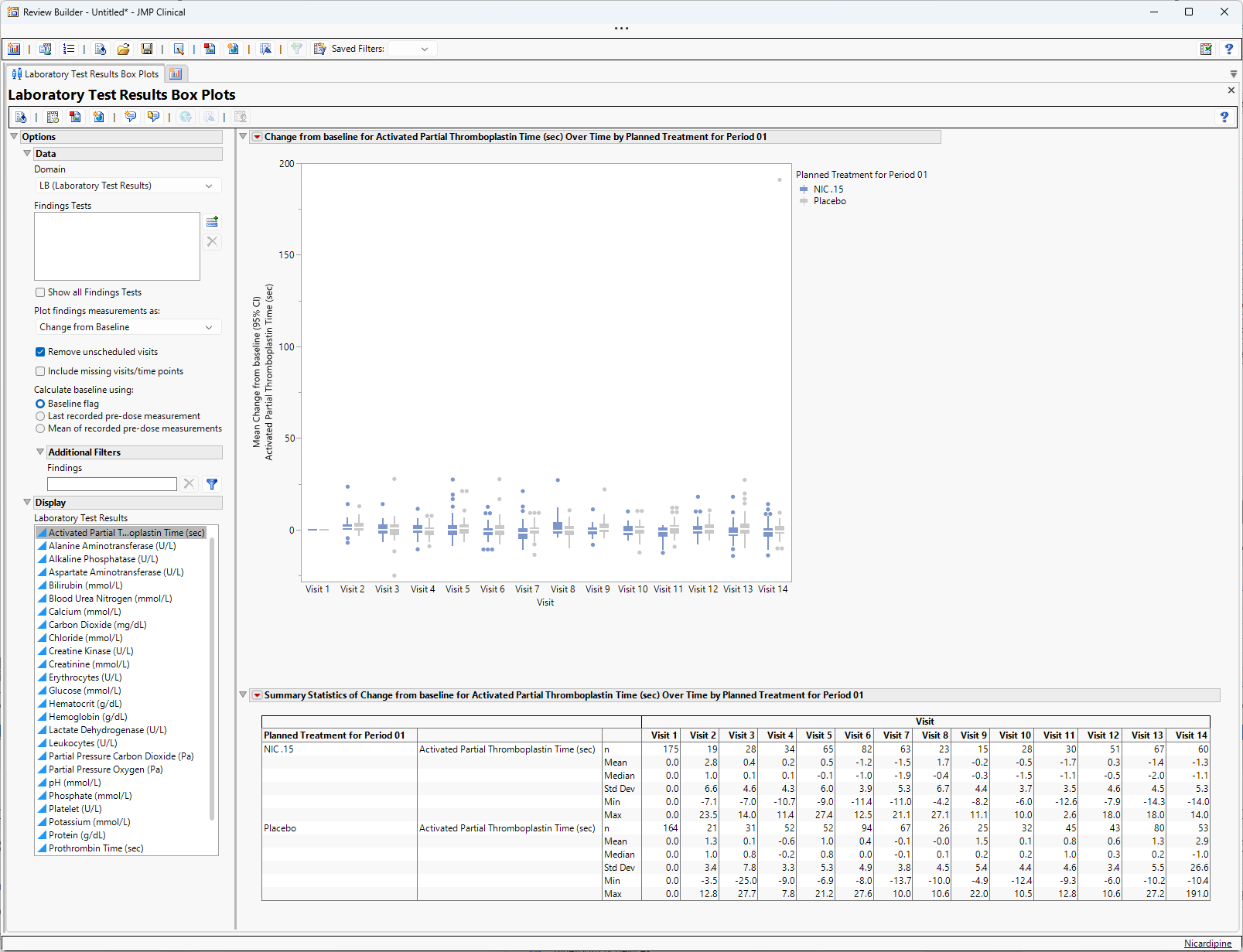
|
| All other options set to default. | |||
Laboratory Test Results (LB) is the selected domain, unscheduled visits have been excluded, and the baseline value is calculated based on the baseline flag. Change from baseline is the selected finding measurement.
This example, which corresponds to Example 1 in the Findings Time Trends Report documentation, summarizes changes from baseline in Blood Urea Nitrogen (BUN). The plotted distributions and summary statistics in this report help characterize patterns and evaluate within-subject change-from-baseline BUN values across visits and between treatment groups. Individual subjects can be identified from the plots to allow further exploration of the subject’s safety profile, findings, or other outcomes experienced during the trial.
Figure 1: Box Plots showing BUN Change from Baseline
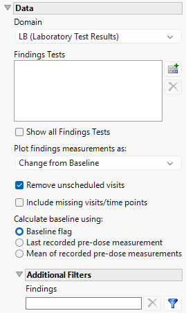
Figure 1 displays the distribution of change-from-baseline BUN values at each follow-up visit. We observe numerous outlying observations in the upper portion of the distributions, representing subjects who experienced large changes from baseline in BUN at various follow-up visits. These subjects may warrant additional review to determine whether the changes are associated with renal impairment, adverse events, concomitant medications, or other clinically relevant factors. These large positive changes from baseline can be observed for subjects in both treatment groups. Hovering over an outlier at Visit 14 identifies a subject in the Nicardipine group with a change-from-baseline BUN value of 43.554 mmol/L. As part of a safety review, it may be useful to evaluate this subject’s renal markers (for example creatinine and eGFR) to better understand the observed change and its relationship to adverse events, drug exposure, concomitant medications and the overall subject profile. TheAcute Kidney Injury report and the Patient Profiles report may be helpful in providing additional insights into the safety profile for this subject or other subjects having unusual change-from-baseline values. The upward shift in the median lines and boxes across visits suggests increasing BUN change-from-baseline values over time, particularly in the Nicardipine group, while the wider interquartile ranges indicate increasing variability among subjects. These interpretations and observations are not based on statistical tests for significance, but may lead to more formal statistical testing, as deemed appropriate, by those conducting the trial. When interpreting changes across visits, reviewers should also consider changes in sample size, as later visits may include fewer subjects than earlier visits.
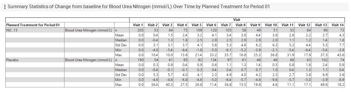
Accompanying the plot in this report is a table (Figure 2) summarizing the min, max, median, mean, standard deviation and sample size (n) for the change-from-baseline BUN at each visit for each treatment group. The mean change from baseline ranges from 0.4 mmol/L to 4.4 mmol/L over the follow-up period in the Nicardipine group. For the Placebo group, the mean change ranges between 0.3 and 2.4 mmol/L across the study. Because outliers can substantially influence the mean, the median may provide a more robust summary for comparing treatment groups. The median change across the visits ranged from -0.4 to 2.9 mmol/L in the Nicardipine group, compared to a range from 0.3 to 2.4 mmol/L in the Placebo group, suggesting a gradual increase in BUN values over time within both groups. The sample sizes vary across follow-up visits which is worth noting as well and may reflect subject discontinuation, missed visits, or incomplete follow-up assessments. Related reports that can support further investigation include the Study Flow Diagram, Study Visits report, and Missing Findings report
Figure 2: Stats Table for BUN Change from Baseline.
Example 2: Mean Diastolic Blood Pressure Over Time by Treatment
 View/Hide Details.
In this example, report options were set as shown in the following table:
| Option Type | Option | Setting | |
|---|---|---|---|
| Data | Domain | VS (Vital Signs) | 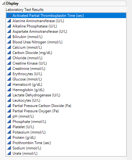
|
| Plot findings measurements as: | Observed Result | ||
| Removed unscheduled visits | unchecked | ||
| Display | Vital Signs | Diastolic Blood Pressure (mmHg) | |
| All other options set to default. | |||
This example uses the Findings Box Plot Report to evaluate the Diastolic Blood Pressure (DBP in mmHg) measured at each visit during the study. The plotted distributions and summary statistics help characterize patterns in DBP within and between treatment groups. Observed outliers and extreme values can lead to further investigations as they pertain to the safety profile for individual subjects on the study.
Figure 3: Observed DBP Over Time
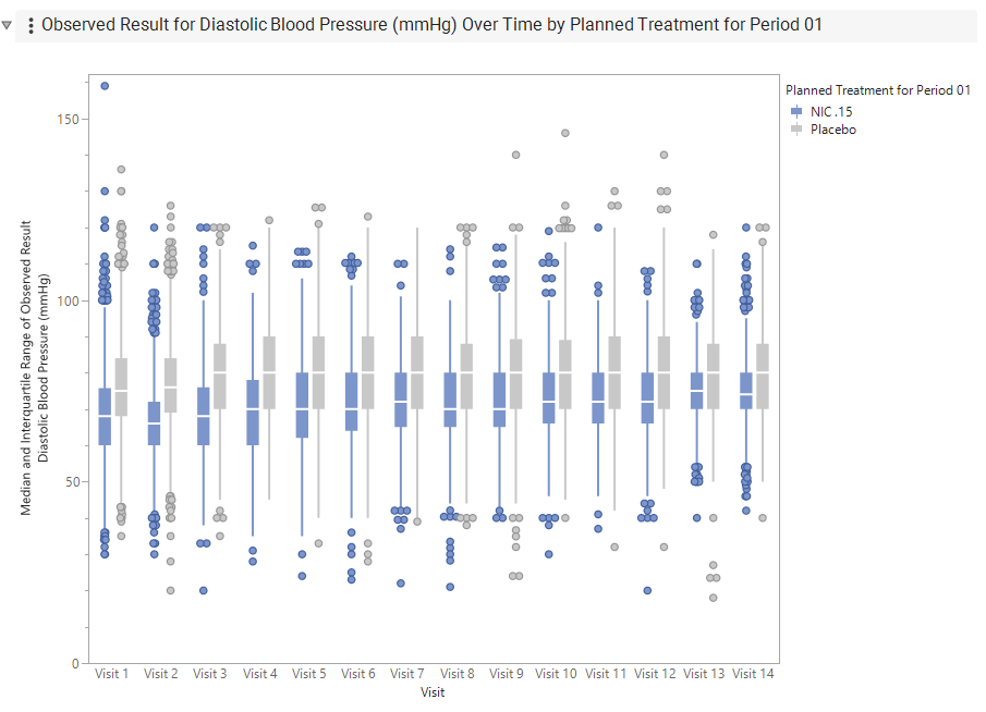
From the plot (Figure 3) we observe a considerable number of outliers, both on the upper and lower ends of the distributions, for example, DBP observed below 40 mmHg and above 100 mmHg. At Visit 1, which represents the baseline visit, there appears to be a modest imbalance between the Nicardipine group and the Placebo group; DBP values appear to be lower in the Nicardipine group compared to the Placebo group. The trend for the Nicardipine group to show relatively lower DBP compared to the Placebo group continues across all the visits in the study.
Figure 4: Summary Statistics on Observed DBP Over Time
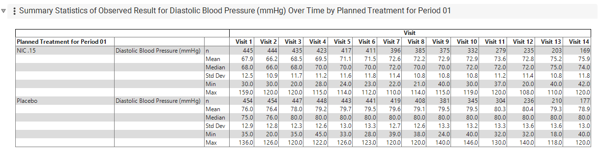
From the summary statistics (Figure 4) we observe at baseline, the median DBP in the Nicardipine group is 68.0 mmHg, compared to 76.0 mmHg in the Placebo group. Across the post-baseline visits, in the Nicardipine group, the mean DBP ranges from 66.2 mmHg to 75.9 mmHg, compared to the Placebo group with mean DBP between 76.4 mmHg to 80.4 mmHg.
To explore whether the nominally lower DBP observed in the Nicardipine group at post-baseline visits is an artifact of the lower initial baseline DBP, we can switch to evaluate the change from baseline for subjects at each visit. This is done by setting the Findings Measurement option to Change from baseline. The resulting change from-baseline graph is shown in Figure 5, below.
Figure 5: Change from Baseline in DBP Over Time
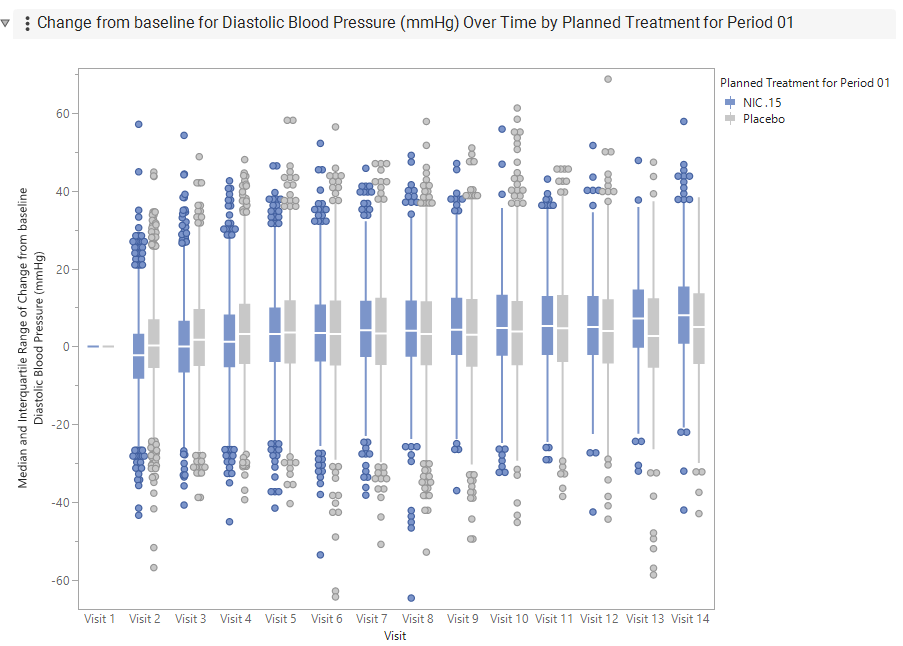
After choosing the Change from Baseline measurement, differences between treatment groups appear to be very minimal. This observation suggests that the apparent difference in post-baseline DBP between treatment groups appearing in Figure 3 may be largely attributable to the imbalance which existed in the treatment groups at baseline.
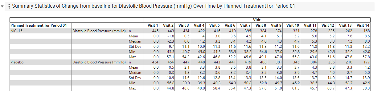
The summary statistics for change-from-baseline DBP values (Figure 6) provide additional details on the mean and median change from baseline in each treatment group. The number of DBP observations at Visits 13 and 14 (i.e., between 168 and 210) is substantially less than the numbers at Visits 2 and 3 (between 443 to 454), suggesting increased rates of missed visits, study discontinuation, or both at later visits in the trial. Related reports that can support further investigation include the Study Visits report,Disposition Distribution report, and Exposure Summary report.
Figure 6: Summary Statistics on Change from Baseline in DBP Over Time
Options
Data
Treatment or Comparison Variable
View/Hide Details.
Specifies the variable used to define the groups to be comparec in the report. This variableis typically a planned or actual treatment variable, such as ARM, ACTARM, TRTxxA, or TRTxxP, but it can also be another variable that defines meaningful comparison groups, such as SEX or RACE.
Select None to display the data without grouping by a treatment or comparison variable.
Domain
View/Hide Details.
Use this widget to specify whether to analyze measurements from either the Electrocardiogram (EG), Laboratory (LB), or Vital Signs (VS) findings domains.
LB is selected by default.
Findings Tests
View/Hide Details.
Use this widget to select specific Findings tests. If you leave this field blank, all tests are run.
| 8 | Click  to open the Add window (shown below) that lists available test names (shown below). to open the Add window (shown below) that lists available test names (shown below). |
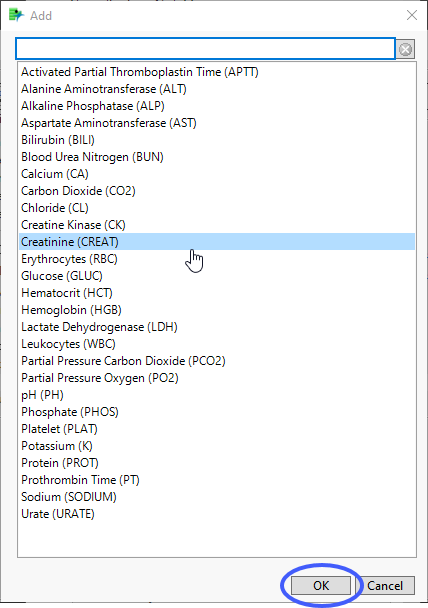
| 8 | Select the desired test(s) and click to add them to the text box. |
Show all Findings Tests
View/Hide Details.
Check this box will show all the graphs for every findings tests instead of one graph with a column switcher.
This box is checked by default.
By Variables
View/Hide Details.
Use this field to specify one or more By variables from ADSL to use in your analysis.

Selecting a By variable will split the bar chart and tabulate by the grouping variables selected in this option as well as by the variable selected for the comparison or treatment variable.
By Variables
By variables are optional (in most reports)variable specifications whose values define groups of observations, such as hour, month, or year. BY variables can enable analyses to be performed separately on different groups as defined by that variable. Choosing a BY variable such as gender (ADSL variable = SEX), for example, groups the subjects by gender and conducts two separate analyses: one for males and one for females.
Alternatively, specifying a BY variable enables you to animate an image so that you can see how response values change according to some grouping, like over time.
To Specify One or More By Variables:
| 8 | Click to open the Add window (shown below) that lists each variable contained in domain and SUPPxx (if merged) specific to this report |
Note: In Demographics Distribution only, variables are taken from ADSL, in addition to the report-specific DS and SUPPPDS (if available) data sets.
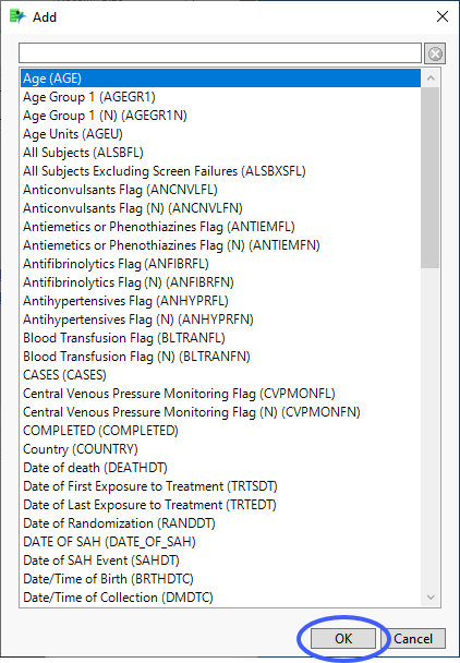
| 8 | Select the variables you want to include in the analysis and click to add those variables to the text box. |
In this example, AGE Group 1, RACE, and SEX were selected and added.
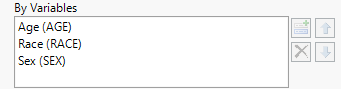
Note: If no BY variables are specified, the analysis is conducted across all the subjects
Plot findings measurements as:
View/Hide Details.
Use this widget to specify whether to plot the results either as observed or how they relate to the baseline measurement.
Available options are listed in the following table:
|
Option |
Description |
|
Observed result |
Plots observed values of the xxSTRESNvariable at or within time points or specified time periods. |
|
Change from baseline |
Plots the change from the findings baseline measurements. |
|
Percent change from baseline |
Plots 100*((xxSTRESN - Baseline)/Baseline) across trial time points. |
|
Percent of baseline |
Plots 100*(xxSTRESN/Baseline). |
Remove unscheduled visits
View/Hide Details.
You might or might not want to include unscheduled visits when you are analyzing findings by visit.
By default, this box is checked. When it is checked, records are excluded from the analysis if the VISIT variable exists and contains the text "unscheduled" for those records. If the box is not checked all records are included regardless of the VISIT status.
For some reports, you may have to specify Visits as the Time Scale to enable this field.
Include missing visits/time points
View/Hide Details.
Check the box to include missing visits/time points in the plots and tables.
Calculate baseline as:
View/Hide Details.
Use this widget to use the flagged baseline record, last recorded pre-dose measurement or the mean of all the measurements taken during the baseline time window as the baseline measurement.
By default, the flagged baseline record is used.
The following test measurements are considered when forming the baseline measurement:
| • | those flagged as baseline, and |
| • | those taken prior to Study Day 1 |
Choose Last recorded pre-dose measurement to use the last recorded pre-dose test measurement (out of the test measurement pool generated from the above list) as the baseline measurement.
Choose Mean of recorded pre-dose measurements to average these pre-dose test measurements to form the baseline measurement.
Note: When the selected option to calculate baseline is to use the baseline flag and there are two records flagged as baseline, JMP Clinical uses the last record. This differs from JMP Clinical version 8.1, wherein the mean of the flagged baseline values was used.
Snapshot Records to Include
View/Hide Details.
Use this widget to specify which updated snapshot records to include in your analysis. This option is surfaced only in studies where the number of snapshots is greater than 0.
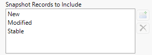
The default state of this option is to show new, modified and stable - effectively all - snapshot records. To see specific records you must remove undesired records from the analysis. For example, to surface only the new records, select both Modified and Stable and click  . Click
  to restore deleted records.
Note: JMP Clinical now relies on the JMP Compare Data Tables platform to detect new records. When duplicate rows appear, the platform evaluates them based on their row order. As a result, records are no longer labeled as Non‑Unique or Previously Non‑Unique, and the corresponding options to include those records have been removed.
Additional Filters - Findings
View/Hide Details.
This filter lets you restrict your analysis to only those subjects that meet specific criteria at the level of the specified Findings domain (EG, LB, or VS) .

This filters uses JMP WHERE clauses to Select Rows that meet the specified criteria. To use this filter, you must enter the JSL (JMP Scripting Language) expressions that constitute the WHERE clause in the appropriate text box for specific filtering of findings. Note: This is an advanced concept that not only requires some basic knowledge of the JSL where clause syntax (similar to, but different from, SQL), but also an understanding of the exact variables in the tables in the study.
Risk indicators are calculated using this subset only.
To specify a Findings filter:
| 8 | Click  to open the Where Clause Builder to construct the desired filter. to open the Where Clause Builder to construct the desired filter. |
| 8 | Click  to clear the filter. to clear the filter. |
Note: To filter subjects with a specific event or finding, one could also use the Subpopulation Builder on any domain of interest. For example, filter to all subjects that exhibit cardiac failure ( :Customized Query 01 Name == "Cardiac failure" ) and run all reports on those.
Display
Test Results/Vital Signs
View/Hide Details.
This option lists all of the tests performed over the course of the study. The list is specific to the selected Findings domain and changes when you change the selected domain.
| 8 | Select one or more tests to display only the results for the selected domain(s). |
Action Buttons
Action buttons provide you with an easy way to drill down into your data. The following action buttons are generated by this report:
Click here to display the list and description of the Report Action buttons..
| • | Click  to rerun the report using default settings. to rerun the report using default settings. |
| • | Click  to view the associated data tables. Refer to Show Tables for more information. to view the associated data tables. Refer to Show Tables for more information. |
| • | Click  to generate a standardized PDF- or RTF-formatted report containing the plots and charts of selected sections. to generate a standardized PDF- or RTF-formatted report containing the plots and charts of selected sections. |
| • | Click  to generate a JMP Live report. Refer to Create Live Report for more information. to generate a JMP Live report. Refer to Create Live Report for more information. |
| • | Click  to take notes, and store them in a central location. Refer to Add Notes for more information. to take notes, and store them in a central location. Refer to Add Notes for more information. |
| • | Click  to read user-generated notes. Refer to View Notes for more information. to read user-generated notes. Refer to View Notes for more information. |
| • | Select one or more subjects, then click  to apply the Review Subject Filter and filter all reports in the review builder on the selected subjects. to apply the Review Subject Filter and filter all reports in the review builder on the selected subjects. |
| • | Select a group of subjects and click  to specify Derived Population Flags that enable you to distinguish the selected group of subjects from the general population. to specify Derived Population Flags that enable you to distinguish the selected group of subjects from the general population. |
| • | Select one or more points (from the same visit or different visits) on the box plot and click  to surface a table listing the findings results for the selected subject(s) from the selected visit(s). to surface a table listing the findings results for the selected subject(s) from the selected visit(s). |
Default Settings
Refer to Set Study Preferences for default Subject Level settings.