The Individual Detail Reports option displays a capability report for each variable in the analysis.
Figure 11.14 shows the Individual Detail Report for PNP1 from the Semiconductor Capability.jmp sample data table as described in Example of the Process Capability Platform with Normal Variables.
Figure 11.14 Individual Detail Report
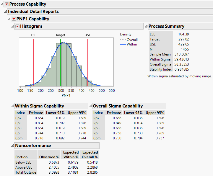
The Individual Details report for a variable with a normal distribution shows a histogram, process summary details, and capability and nonconformance statistics. The histogram shows the distribution of the values, the lower and upper specification limits and the process target (if they are specified), and one or two curves showing the assumed distribution. The histogram in Figure 11.14 shows two normal curves, one based on the overall estimate of standard deviation and the other based on the within-subgroup estimate.
When you fit your process with a normal distribution, the Process Summary includes the Stability Index, which is a measure of stability of the process. The stability index is defined as follows:
Figure 11.15 shows the Individual Detail Report for Process 1 from the Process Measurements.jmp sample data table as described in Example of the Process Capability Platform with Nonnormal Variables.
Figure 11.15 Individual Detail Report for Process 1
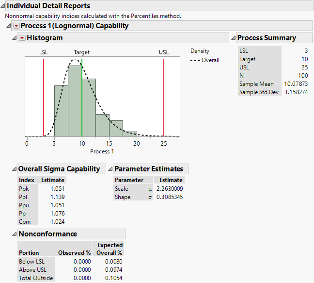
The report also shows a Parameter Estimates report if you selected a nonnormal parametric distribution or a Nonparametric Density report if you selected a Nonparametric fit. See Parameter Estimates and Nonparametric Density.
Shows or hides the control panel for comparing distributions for the process. See Compare Distributions.
Shows or hides capability indices (and confidence intervals) based on the overall (long-term) sigma.
The estimates for all except the Johnson family distributions are obtained using maximum likelihood. For details about Johnson family fits, see Johnson Distribution Fit Method.
The parameters and probability density functions for the normal, beta, exponential, gamma, Johnson, lognormal, and Weibull distributions are described in Capability Indices for Nonnormal Distributions: Percentile and Z-Score Methods. These are the same parameterizations used in the Distribution platform, with the exception that Process Capability does not support threshold parameters. See Distributions in the Basic Analysis book.
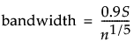
(Available when Nonparametric is selected as the distribution.) Shows or hides the Nonparametric Density report, which gives the kernel bandwidth used in fitting the nonparametric distribution. The kernel bandwidth is given by the following, where n is the number of observations and S is the uncorrected sample standard deviation:
|
–
|
Figure 11.16 shows the Compare Distributions report for Process 1 in the Process Measurements.jmp sample data table. The Selected distribution, which is Lognormal, is being compared to a Normal distribution. The Comparison Details report shows fit statistics for both distributions.
You can obtain probability plots by selecting the Probability Plots option from the Compare Distributions red triangle menu. The points in the probability plot for the normal distribution in Figure 11.16 do not follow the line closely. This indicates a poor fit.
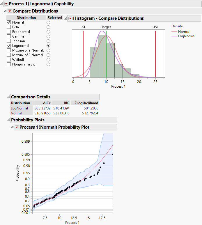
For each distribution, gives AICc, BIC, and -2Loglikelihood values. See Likelihood, AICc, and BIC in the Fitting Linear Models book. (Not available for a Nonparametric fit.)
Shows or hides a report that displays probability plots for each parametric distribution that you fit. See Figure 11.16. An observation’s horizontal coordinate is its observed data value. An observation’s vertical coordinate is the value of the quantile of the fitted distribution for the observation’s rank. For the normal distribution, the overall estimate of sigma is used in determining the fitted distribution.
Shows or hides confidence limits that have a simultaneous 95% confidence level of containing the true probability function, given that the data come from the selected parametric family. These limits have the same estimated precision at all points. Use them to determine whether the selected parametric distribution fits the data well. See Nair (1984) and Meeker and Escobar (1998).
When possible, the intervals are computed by expressing the parametric distribution F as a location-scale family, so that F(y) = G(z), where z = (y - μ)/σ. The approximate standard error of the fitted location-scale component at a point is computed using the delta method. Using the standard error estimate, a Wald confidence interval for z is computed for each point. The confidence interval for the cumulative distribution function F is obtained by transforming the Wald interval using G. Note that, in some cases, special accommodations are required to provide appropriate intervals near the endpoints of the interval of process measurements.