After selecting database tables (and joining them if necessary), click Build Query to open the Query Builder window. You can continue to refine the query by selecting which columns to include and specifying criteria for sampling and filtering. You can also save the query to edit and run again later.
The columns from all database tables appear in the Available Columns list. Prefixes such as t1 and t2 (also called aliases) associate each column with the corresponding database table.
To skip the Query Builder step and import all data, click Import Now instead.
Note: The JMP Query Builder in the Tables menu provides many of the same options but lets you query and join JMP data tables. See Query and Join Data Tables with JMP Query Builder in Reshape Data for details.
|
1.
|
Select File > New > Database Query, connect to the database, and select the SQBTest schema. (See Connect to a Database for details.)
|
|
2.
|
|
3.
|
|
4.
|
Click Build Query to show the Query Builder window.
|
|
5.
|
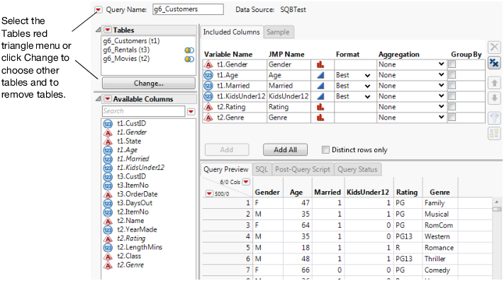
In the Available Columns box, select t1.Gender, t1.Age, t1.Married, t1.KidsUnder12, t2.Rating, and t2.Genre.
|
|
6.
|
Click Add on the Included Columns tab.
|
Figure 2.33 Selected Columns
|
7.
|
Select the SQL tab below the columns to view the SQL statements for your query. This code is saved as a data table property after you run the query.
|
|
8.
|
Click Save in the lower right corner.
|
Your work is saved as g6_Customers.jmpquery, which you can open later to return to this point or to run the query.
|
9.
|
Click Run Query to import the data.
|
|
•
|
To rename an alias, right-click the table in the Select Tables for Query window and select Change Alias. Aliases are not case sensitive.
|
|
•
|
The query runs in the background unless you deselect Run queries in the background when possible from the Query Builder ODBC preferences. You can also check the progress of all ODBC queries by selecting View > Running Queries.
|
|
•
|
Deselect Update preview automatically if the preview loads too slowly. Click Update below the Query Preview tab to update the data view. Consider changing the Preview options in the JMP Query Builder preferences if you frequently work with large databases. Consider limiting the maximum number of rows that can be previewed. In the JMP Query Builder preferences, change the value of Maximum number of rows for previews.
|
|
•
|
To omit duplicate rows from the database, select Distinct rows only on the Included Columns tab.
|
If you add a JMP 13 feature to a query, that query will no longer load in JMP 12. If you are using JMP 13, but you need to create queries that will still run in JMP 12, select Keep this query compatible with JMP 12 in the Query Builder Preferences. After you select the option, features that create compatibility problems are hidden in Query Builder.
You can create a new column from existing columns. You might calculate the mean for two columns and store the mean in a new column. Date-time values might be in the wrong format. From the Available Columns red triangle menu, select Add Computed Column, and create the new column in the formula editor.
|
1.
|
Select File > New > Database Query, connect to the database, and select the SQBTest schema. (See Connect to a Database for details.)
|
|
2.
|
In the Select Tables for Query window, select g6_Rentals as the Primary table and g6_Movies as the Secondary table.
|
|
3.
|
Click Build Query to show the Query Builder window.
|
|
4.
|
From the Available Columns red triangle menu, select Add Computed Column.
|
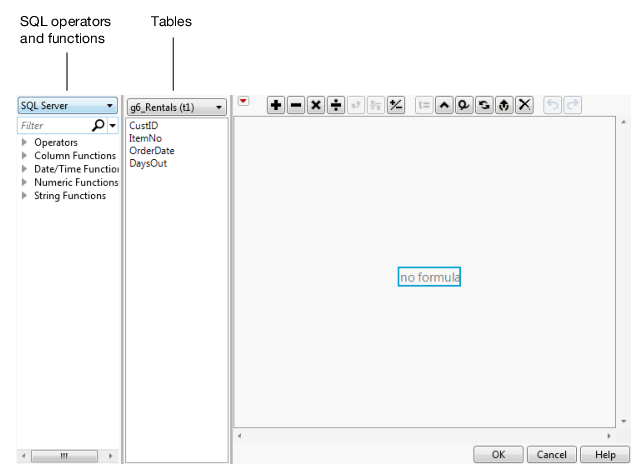
The Computed Column window appears (Figure 2.34). The window contains the JMP Formula Editor.
Figure 2.34 Computed Column Window with Formula Editor
|
–
|
Operators and functions are provided in the list on the left side of the Formula Editor (Figure 2.34). In some instances, you might need to change the server type based on your database.
|
|
–
|
The Operators list does not provide a Concatenate (||) operator. You must type the formula in the Formula Editor box.
|
|
5.
|
 button.
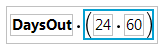
Figure 2.35 Computed Column

Figure 2.36 First Portion of the Formula
 button.
|
8.
|
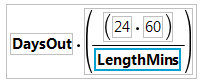
Figure 2.37 Second Portion of the Formula
|
9.
|
Click OK.
|
|
10.
|
Right-click the column and select Rename Column.
|
|
11.
|
|
12.
|
|
13.
|
Note: Aggregation support is based on your database. See the database documentation for more information.
|
1.
|
Select File > New > Database Query, connect to the database, and select the SQBTest schema. (See Connect to a Database for details.)
|
|
2.
|
In the Select Tables for Query window, select g6_Movies as the Primary table and g6_Rentals as the Secondary table.
|
|
3.
|
Click Build Query to show the Query Builder window.
|
|
4.
|
|
5.
|
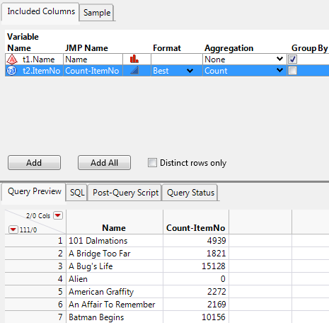
The Group By check box is selected for t1.Name (Figure 2.38). All instances of a specific movie name will be grouped into one row.
Figure 2.38 Grouped Columns
|
6.
|
Click Run Query to import the data.
|
|
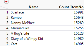
7.
|
Figure 2.39 Sorted Count-ItemNo Column
|
•
|
To clear the grouped rows, select None from the column’s Aggregation list.
|
Suppose that you want to import a sample of the data. In this example, you select 5,000 random rows.
|
1.
|
Select File > New > Database Query, connect to the database, and select the SQBTest schema. (See Connect to a Database for details.)
|
|
2.
|
In the Select Tables for Query window, select g6_Rentals as the Primary table and g6_Movies as the Secondary table.
|
|
3.
|
Click Build Query to show the Query Builder window.
|
|
4.
|
Click the Add All button on the Included Columns tab.
|
|
5.
|
|
6.
|
Select Random N Rows and type 5,000.
|
|
7.
|
Click Run Query to import the data.
|
|
•
|
To add individual columns to the Included Columns tab, right-click the column and select Include Column or click the Add button.
|
Add filters to import a subset of values from the selected filters into the data table. Some filters are not available if the query is compatible with JMP 12. See Maintain Compatibility with JMP 12 for details.
Age > 14 matches ages that are greater than 14.
12 ≤ Age ≤ 17 matches ages that are between 12 and 17.
Either NULL or not NULL matches missing values and non-missing values.
( ( ( t2.Gender IN ( 'F' ) ) AND ( (t2.Age >= 20) AND (t2.Age <= 50) ) ) )
Note: List Box, Manual List, and Check Box List include a Not in list option that enables you to retrieve rows that do not match the selected values.
Matches a string that contains or does not contain the specified value. Contains Comedy OR Romance matches Comedy and Romance.
Matches a string that is similar to or not similar to the specified value. Supports the % wildcard (zero or more characters) and _ wildcard (exactly one character).
Genre Like %com matches any number of characters before “com”, as in “RomCom”. To also match “Comedy”, use %com% or Contains com.
Matches the specified column value. Select the table and then select the columns. The Select non-matching option enables you to filter all rows except for the selected rows. See Import Matching Data from an Existing Data Table for an example.
|
1.
|
Select File > New > Database Query, connect to the database, and select the SQBTest schema. (See Connect to a Database for details.)
|
|
2.
|
In the Select Tables for Query window, select g6_Rentals from the Available Tables list, and then click Primary.
|
|
3.
|
|
4.
|
Click Build Query to show the Query Builder window.
|
|
5.
|
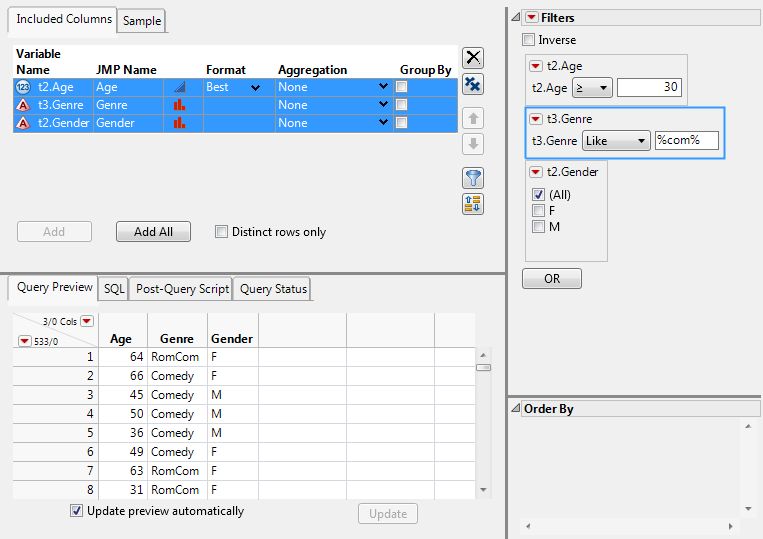
In the Available Columns box, select t2.Gender, t2.Age, and t3.Genre, and then click Add on the Included Columns tab.
|
|
6.
|
 .
.|
7.
|
Set the t2.Age filter to ≥ 30.
|
|
8.
|
The % wildcards match any number of characters before and after “com”. On the Query Preview tab, notice that movies in both the RomCom and Comedy genres are shown (Figure 2.40).
Figure 2.40 Selecting Filters
|
9.
|
In the Filters red triangle menu, select All Prompt on Run.
|
|
10.
|
Click Run Query.
|
|
11.
|
In the Query Prompts window, click OK to apply the preselected filters and import the data.
|
|
•
|
|
–
|
The Query Builder preference called Retrieve category levels for tables whose size cannot be determined is selected by default so that JMP automatically retrieves the levels. If you deselect the preference, the Contains fallback filter type in the Query Builder preferences is selected.
|
|
–
|
If the categorical column has more than 1 million rows, JMP does not automatically retrieve the unique category levels for the filtered column. The Query Builder preference called Maximum rows in table for which category levels will be automatically retrieved supports a minimum of -1 (no limit) and a maximum value of 1 billion rows.
|
|
•
|
The default filter for categorical columns is a list box unless the Keep this query compatible with JMP 12 Query Builder preference is selected.
|
|
1.
|
|
2.
|
Select File > New > Database Query, connect to the database, and select the SQBTest schema. (See Connect to a Database for details.)
|
|
3.
|
In the Select Tables for Query window, select g5_AIRLINE_ONTIMEPERF from the Available Tables list, and then click Primary.
|
|
4.
|
Click Build Query to show the Query Builder window.
|
|
5.
|
Click Add All on the Included Columns tab.
|
|
6.
|
|
7.
|
From the t1.TailNum red triangle menu in the Filters column, select Filter Type, and then select Match Column Values.
|
|
8.
|
|
9.
|
|
10.
|
Click Run Query to import the data.
|
The data table includes only data for rows that are in the Tail Number column.
|
1.
|
|
2.
|
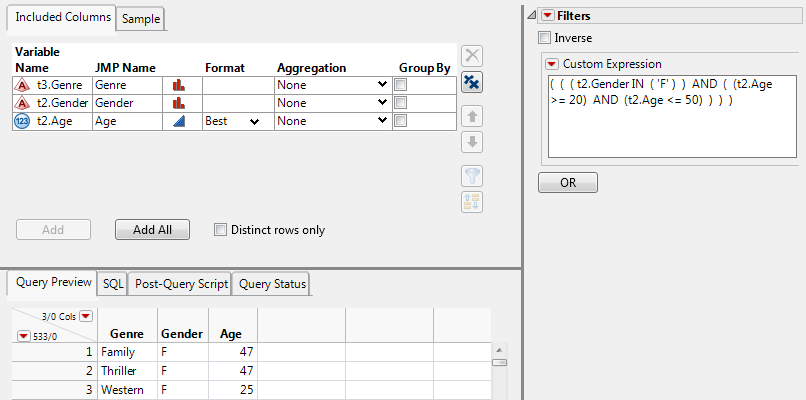
From the Filters red triangle menu, select Add Custom Expression.
|
( ( ( t2.Gender IN ( 'F' ) ) AND ( (t2.Age >= 20) AND (t2.Age <= 50) ) ) )
Figure 2.41 Writing a Custom Filter Expression
|
1.
|
Select File > New > Database Query, connect to the database, and select the SQBTest schema. (See Connect to a Database for details.)
|
|
2.
|
|
3.
|
Click Build Query to show the Query Builder window.
|
|
4.
|
On the Included Columns tab, click Add All.
|
|
5.
|
 .
.
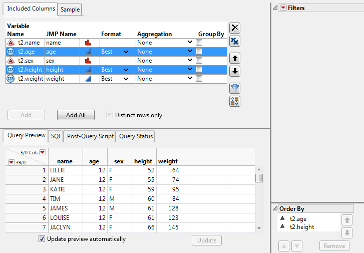
Figure 2.42 Selecting the Order By Columns
|
6.
|
In the Order By outline, select t1.height and then click Sort the values in descending order
 below the columns. below the columns. |
The height column is sorted from tallest to shortest.
|
7.
|
 .
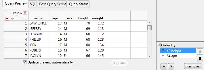
.The height column is sorted first. Values in the age column are sorted within each level of height. For a height of 68, age is sorted from 14 to 17.
Figure 2.43 Result of Reordering Columns
On the Query Status tab, view the status of a query as it runs in the background. The query name, SQL statements, and number of processed records appear. You can stop a query at any time and view only the processed records. To view background queries from other JMP windows, select View > Running Queries. The status details are unavailable if you deselect Run queries in the background when possible from the Query Builder preferences.
Distribution( Column( :age, :gender ) );