|
1.
|
Select DOE > Custom Design.
|
|
2.
|
Type 2 next to Add N Factors.
|
|
3.
|
Click Add Factor > Continuous.
|
|
4.
|
Click Continue.
|
|
5.
|
Click RSM.
|
Quadratic and interactions terms for X1 and X2 are added to the model. Because you added RSM terms, the Recommended optimality criterion changes from D-Optimal to I-Optimal. You can see this later in the Design Diagnostics outline.
Note: Setting the Random Seed in step 6 and Number of Starts in step 7 reproduces the exact results shown in this example. In constructing a design on your own, these steps are not necessary.
|
6.
|
(Optional) From the Custom Design red triangle menu, select Set Random Seed, type 383570403, and click OK.
|
|
7.
|
|
8.
|
Click Make Design.
|
Figure 4.40 I-Optimal Design
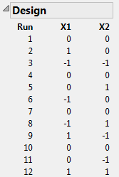
In this I-optimal design, runs 1, 4, 7, and 10 are at the center point (X1 = 0 and X2 = 0). I-optimal designs tend to place more runs in the center (and consequently fewer runs at the extremes) of the design space than do D-optimal designs. You can compare this design to the D-optimal design shown in Figure 4.42.
|
9.
|
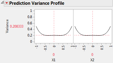
Figure 4.41 Prediction Variance Profile for I-Optimal Model
|
10.
|
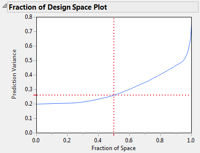
Open the Fraction of Design Space Plot outline.
|
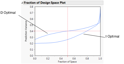
The Fraction of Design Space Plot appears on the left in Figure 4.44. When the Fraction of Space is 0.95, the vertical coordinate of the blue curve is about 0.5. This means that for about 95% of the design space, the relative prediction variance is below 50% of the error variance.
|
1.
|
In the Custom Design window containing your I-optimal design, from the Custom Design red triangle menu, select Save Script to Script Window.
|
|
2.
|
In this new script window, select Edit > Run Script.
|
|
4.
|
From the red triangle next to Custom Design, select Optimality Criterion > Make D-Optimal Design.
|
|
5.
|
(Optional) From the Custom Design red triangle menu, select Set Random Seed, type 383570403, and click OK.
|
|
6.
|
Click Make Design.
|
Figure 4.42 D-Optimal Design
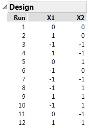
In this D-optimal design, run 1 is the only run at the center point. D-optimal designs tend to place more runs at the extremes of the design space than do I-optimal designs. Recall that the I-optimal design had four center runs (Figure 4.40).
|
7.
|
Figure 4.43 Prediction Variance Profile for D-Optimal Model
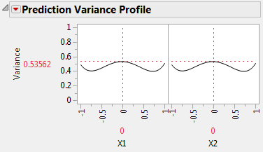
At the center of the design region, the relative prediction variance is 0.53562, as compared to 0.208333 for the I-optimal design (Figure 4.41). This means that the relative standard error is 0.732 for the D-optimal design and 0.456 for the I-optimal design. All else being equal, at the center of the design region, confidence intervals for the expected response based on the D-optimal design are about 60% wider than those based on the I-optimal design.
The Design outline shows that the D-optimal design has nine design points, one for every combination of X1 and X2 set to -1, 0, 1. The D-optimality criterion attempts to keep the relative prediction variance low at each of these design points. Explore the variance at the extremes of the design region by moving the sliders for X1 and X2 to -1 and 1. Note that the variance at these extreme points is usually smaller than the variance for the I-optimal design at these points.
|
8.
|
|
9.
|
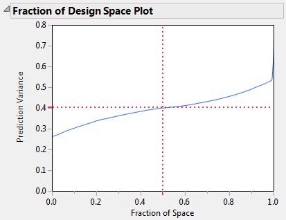
Right-click in the Fraction of Design Space Plot for your I-optimal design. Select Edit > Copy Frame Contents.
|
|
10.
|
Right-click in the Fraction of Design Space Plot for your D-optimal design. Select Edit > Paste Frame Contents.
|
Figure 4.45 Fraction of Design Space Plots Superimposed