Bayes Plot Report
The Bayes Plot report gives another approach to determining which effects are active. This report helps you compute posterior probabilities using a Bayesian approach. This method, due to Box and Meyer (1986), assumes that the estimates are a mixture from two distributions. The majority of the estimates, corresponding to inactive effects, are assumed to be pure random normal noise with variance σ2. The remaining estimates, the active ones, are assumed to come from a contaminating distribution that has a variance K times larger than σ2.
Term
Gives the model term corresponding to the parameter estimate.
Estimate
Gives the parameter estimate. The Bayes plot is constructed with respect to estimates that have estimated standard deviation equal to 1. If the estimates are not correlated, the t-Ratio is used. If the estimates are correlated, the Orthog t-Ratio is used.
Prior Prob
Enables you to specify a probability that the estimate is nonzero (equivalently, that the estimate is in the contaminating distribution). Prior probabilities for estimates are usually set to equal values. The commonly recommended value of 0.2 appears initially, though you can change it.
K Contam
The value of the contamination coefficient, representing the ratio of the contaminating distribution variance to the error variance. K is commonly set to 10, which is the default value.
Std Err Scale
If there are degrees of freedom for an estimate of standard error, this value is set to 1. JMP uses this value because the estimates used in the report are transformed and scaled to unit variance. The value is set to 0 for a saturated model with no estimate of error. If you specify a different value, think of it in terms of a scale factor of the RMSE estimate.
DFE
Gives the error degrees of freedom.
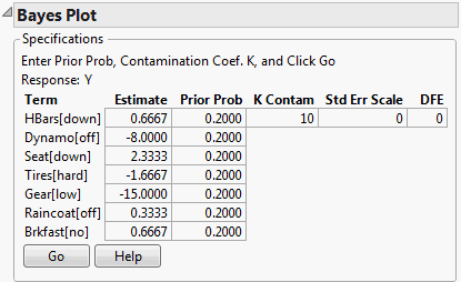
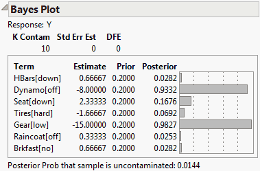
The specifications window, showing default settings for a Bayes Plot for the Bicycle.jmp sample data table, is shown in Figure 3.46. Clicking Go in this window updates the report to show Posterior probabilities for each of the terms and a bar chart (Figure 3.47).
Example of a Bayes Plot
1. Select Help > Sample Data Library and open Bicycle.jmp.
2. Select Analyze > Fit Model.
3. Select Y and click Y.
4. Select HBars through Brkfast and click Add.
5. Click Run.
6. Click the Response Y red triangle and select Effect Screening > Bayes Plot.
Figure 3.46 Bayes Plot Specifications
7. Click Go to calculate the posterior probabilities.
Figure 3.47 Bayes Plot Report
The note beneath the plot in the Bayes Plot report gives the Posterior Prob that the sample is uncontaminated. Posterior Prob is the probability, based on the priors and the data, that there are no active effects whatsoever. The probability is small, 0.0144, indicating that it is likely that there are active effects. The Posterior probability column suggests that at least Dynamo and Gear are active effects.

