Examples
Open the Singularity.jmp sample data table. There is a response Y, four predictors X1, X2, X3, and A, and five observations. The predictors are continuous except for A, which is nominal with four levels. Also note that there is a linear dependency among the continuous effects, namely, X3 = X1 + X2.
Non-Uniqueness of Estimates
To see that estimates are not unique when there are linear dependencies:
1. Select Help > Sample Data Library and open Singularity.jmp.
2. Run the script Model 1. The script opens a Fit Model launch window where the effects are entered in the order X1, X2, X3.
3. Click Run and leave the report window open.
4. Run the script Model 2. The script opens a Fit Model launch window where the effects are entered in the order X1, X3, X2.
5. Click Run and leave the report window open.
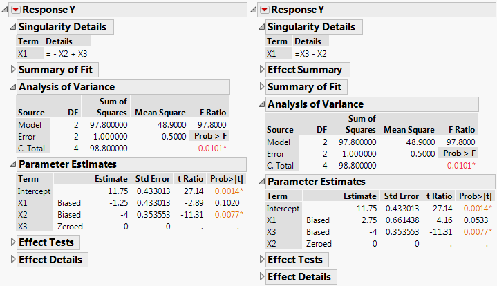
Compare the two reports (Figure 3.66). The Singularity Details report at the top of both reports displays the linear dependency, indicating that X1 = X3 - X2.
Now compare the Parameter Estimates reports for both models. Note, for example, that the estimate for X1 for Model 1 is –1.25 while for Model 2 it is 2.75. In both models, only two of the terms associated with effects are estimated, because there are only two model degrees of freedom. See the Analysis of Variance report. The estimates of the two terms that are estimated are labeled Biased while the remaining estimate is set to 0 and labeled Zeroed.
The Effect Tests report shows that no tests are conducted. Each row is labeled LostDFs. The reason this happens is as follows. The effect test for any one of these effects requires it to be entered into the model last. However, the other two effects entirely account for the model sum of squares associated with the two model degrees of freedom. So there are no degrees of freedom or associated sum of squares left for the effect of interest.
Figure 3.66 Fit Least Squares Reports for Model 1 (on left) and Model 2 (on right)
LostDFs
To gain more insight on LostDFs, follow the steps below or run the data table script Fit Model Report:
1. Select Help > Sample Data Library and open Singularity.jmp.
2. Click Analyze > Fit Model.
3. Select Y and click Y.
4. Select X1 and A and click Add.
5. Set the Emphasis to Minimal Report.
6. Click Run.
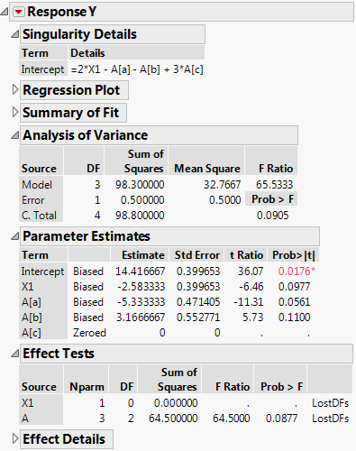
Portions of the report are shown in (Figure 3.67). The Singularity Details report shows that there is a linear dependency involving X1 and the three terms associated with the effect A. (For more information about how a nominal effect is coded, see Details of Custom Test Example). The Analysis of Variance report shows that there are three model degrees of freedom. The Parameter Estimates report shows Biased estimates for the three terms X1, A[a], and A[b] and a Zeroed estimate for the fourth, A[c].
The Effect Tests report shows that X1 cannot be tested, because A must be entered first and A accounts for the three model degrees of freedom. However, A can be tested, but with only two degrees of freedom. (X1 must be entered first and it accounts for one of the model degrees of freedom.) The test for A is partial, so it must be interpreted with care.
Figure 3.67 Fit Least Squares Report for Model with X1 and A