Models
The following table provides the equations for each model in the Path Definition list. For a description of each model, follow the link.
Note: The thumbnail sketch shown to the left of each equation shows a generic plot of the behavior of the location parameter, μ, over time. In the report’s main plot, the plot of the estimated median can differ from the thumbnail based on your selections for Distribution and Transformation.
|
Model |
Equation |
|---|---|
|
μ = b0 + b1 * f(time) |
|
|
μ = b1 * f(time) |
|
|
μ = b0X + b1 * f(time) |
|
|
μ = b0X + b1x * f(time) |
|
|
μ = b1X * f(time) |
|
|
μ = b0 + b1X * f(time) |
|
|
μ = b0 - b1 * Exp[-b2 * Exp[b3 * [Arrhenius(X0) - Arrhenius(X)]] * f(time)] |
|
|
μ = b0 * [1 - Exp[-b1 * Exp[b2 * [Arrhenius(X0) - Arrhenius(X)]] * f(time)]] |
|
|
μ = b0 + b1 * Exp[-b2 * Exp[b3 * [Arrhenius(X0) - Arrhenius(X)]] * f(time)] |
|
|
μ = b0 * Exp[-b1 * Exp[b2 * [Arrhenius(X0) - Arrhenius(X)]] * f(time)] |
|
|
μ = b0 ± Exp[b1 + b2 * Arrhenius(X)] * f(time) |
|
|
μ = b0 ± Exp[b1 + b2 * Log(X)] * f(time) |
|
|
μ = b0 ± Exp[b1 + b2 * X] * f(time) |
Models That Are Linear in Transformed Time
Common Path with Intercept
This model fits a single distribution whose location parameter changes linearly over transformed time. This model fits a common intercept and a common slope, regardless of whether there is an X variable.
Common Path without Intercept
This model fits a single distribution whose location parameter changes linearly over transformed time but whose value at time zero is zero. Based on selections for Distribution and Transformation, the median curve might not be a straight line and might not pass through origin. This model fits a zero intercept and a common slope, regardless of whether there is an X variable.
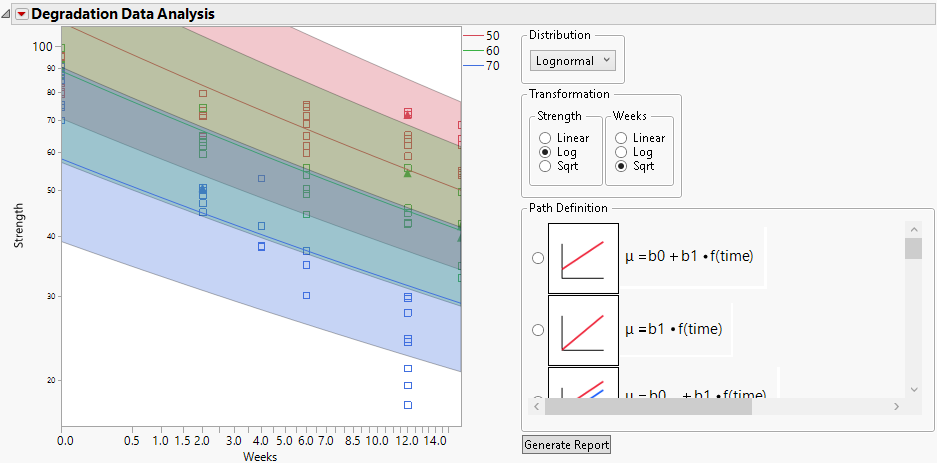
Common Slope
In this model, the location parameters are linear functions of transformed time with separate intercepts for the values of X but a common slope. Based on selections for Distribution and Transformation, the model fits might appear as curves. For example, selecting a Lognormal distribution gives the plot in Figure 8.12.
Figure 8.12 Common Slope Model Using a Lognormal Distribution
Individual Path with Intercept
In this model, the location parameters are linear functions of transformed time with separate intercepts and separate slopes for the values of X.
Individual Path without Intercept
In this model, the location parameters are linear functions of transformed time with zero intercepts and separate slopes for the values of X.
Common Intercept
In this model, the location parameters are linear functions of transformed time with a common intercept and separate slopes for the values of X.
First-Order Kinetics Models
Four first-order kinetics models where the location parameter is a nonlinear function based on an Arrhenius transformation of temperature are provided. Each of these location models fit separate models for each value of the optional explanatory variable X.
When you first select any of these models, you must specify the measurement scale for temperature and a reference temperature value, X0. The specified reference temperature affects the interpretation of b2 in these models. The b2 parameter is the rate constant at X0. The value for X0 is used to construct a time acceleration factor (Meeker and Escobar 1998). If you subsequently select another of the first-order kinetics models or the Arrhenius Rate model (see Arrhenius Rate), the platform remembers and uses these specifications.
First-Order Kinetics Type 1
In this model, b1 and b2 are positive. On a linear scale, the curves have an upper asymptote at b0 as time approaches infinity.
First-Order Kinetics Type 2
In this model, the location parameter is zero at time zero. Both b0 and b1 are positive. On a linear scale, the curves have an upper asymptote at b0 as time approaches infinity. You can think of the Type 2 model as a vertically shifted version of the Type 1 model.
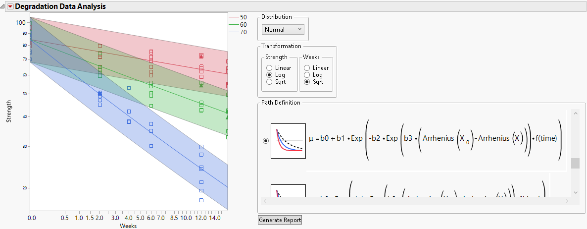
First-Order Kinetics Type 3
In this model, both b1 and b2 are positive. Because of the sign preceding b1 is the opposite of the sign preceding b1 in the Type 1 model, this model is an inverted version of the Type 1 model. On a linear scale, it has a lower asymptote at b0 as time approaches infinity.
Given data exhibiting a negative slope over time, the fitted model can produce a plot similar to Figure 8.13. The figure is for Adhesive Bond.jmp. The selected temperature measurement scale is Celsius and the specified reference temperature under typical use conditions is 35 degrees.
Figure 8.13 Example of First-Order Kinetics Model Type 3
First-Order Kinetics Type 4
This model is a vertically shifted version of the Type 3 model. On a linear scale, the curves have a lower asymptote at 0 as time approaches infinity.
Rate Models
Three models where the location parameter is an exponential function of the transformed X variable are provided. Each of these location models fits common intercept and separate slope models for each value of the optional explanatory variable X. For each of these models, on a linear scale, the location parameter is linear in the transformed time values.
Arrhenius Rate
This model involves an exponential function of the Arrhenius transformation multiplied by transformed time. When you select this model, you are asked to specify the measurement scale for temperature, unless you have already supplied this information.
Polynomial Rate
This model involves an exponential function of a linear function of the log of X multiplied by transformed time.
Exponential Rate
This model involves an exponential function of a linear function of X multiplied by transformed time.