Statistical Details for Capability Analysis
This section contains details about the computation of the statistics in the Capability Analysis report.
Variation Statistics
All capability analyses use the same formulas. Options differ in how sigma (σ) is computed:
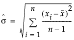
Long Term Sigma
Uses the overall sigma. This option is used for Ppk statistics, and computes sigma as follows:
Note: By default, the capability indices in the Long Term Sigma report use the Cp labeling that is used in the other sigma reports. To use Ppk labeling in the Long Term Sigma report, select the File > Preferences > Platforms > Distribution > PpK Capability Labeling preference.
Control Chart Sigma
Uses a sigma that is determined by the control chart settings.
– If you specify a value for Sigma using the Specify Stats button in the control launch window, the specified value is used for computing capability indices.
– In an IR chart that uses the Moving Range (Average) option, the value for sigma is computed as follows: 
where:
 is the average of the moving ranges.
d2(n) is the expected value of the range of n independent normally distributed variables with unit standard deviation, where n is the value of the Range Span option.
– In an IR chart that uses the Median Moving Range option, the value for sigma is computed as follows:

where:
MMR is the median of the nonmissing moving ranges.
d4(n) is the median of the range of n independent normally distributed variables with unit standard deviation, where n is the value of the Range Span option.
– In an XBar chart that uses the R option, the value for sigma is computed as follows:
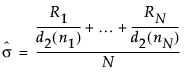
where:
Ri = range of ith subgroup
ni = sample size of ith subgroup
d2(ni) = expected value of the range of ni independent normally distributed variables with unit standard deviation
N = number of subgroups for which ni ≥ 2
– In an XBar chart that uses the S option, the value for sigma is computed as follows:
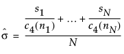
where:
ni = sample size of ith subgroup
c4(ni) = expected value of the standard deviation of ni independent normally distributed variables with unit standard deviation
N = number of subgroups for which ni ≥ 2
si = sample standard deviation of the ith subgroup
Capability Indices for Normal Distributions
This section provides details about the calculation of capability indices for normal data.
For a process characteristic with mean μ and standard deviation σ, the population-based capability indices are defined as follows.
Cp = 
Cpl = 
Cpu = 
Cpk = 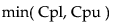
Cpm = 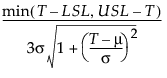
where:
LSL is the lower specification limit.
USL is the upper specification limit.
T is the target value.
For sample-based capability indices, the parameters are replaced by their estimates. The estimate for σ uses the method that you specified in the Capability Analysis window. See Variation Statistics.
If either of the specification limits is missing, the capability indices containing the missing specification limit are reported as missing.
Tip: A capability index of 1.33 is often considered to be the minimum value that is acceptable. For a normal distribution, a capability index of 1.33 corresponds to an expected number of nonconforming units of about 6 per 100,000.
Confidence Intervals for Capability Indices
Note: Confidence intervals for capability indices appear only in the Long Term Sigma report.
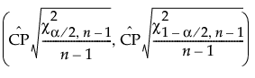
The 100(1 - α)% confidence interval for Cp is calculated as follows:
where:
 is the estimated value for Cp.
 is the (α/2)th quantile of a chi-square distribution with n - 1 degrees of freedom.
n is the number of observations.
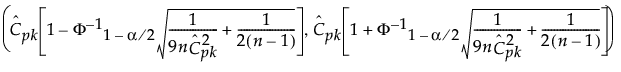
The 100(1 - α)% confidence interval for Cpk is calculated as follows:
where:
 is the estimated value for Cpk.
 is the (1 - α/2)th quantile of a standard normal distribution.
n is the number of observations.
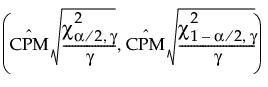
The 100(1 - α)% confidence interval for CPM is calculated as follows:
where:
 is the estimated value for CPM.
 is the (α/2)th quantile of a chi-square distribution with γ degrees of freedom.
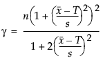
n is the number of observations.
 is the mean of the observations.
T is the target value.
s is the long-term sigma estimate.
Note: The confidence interval for CPM is computed only when the target value is centered between the lower and upper specification limits.
Lower and upper confidence limits for CPL and CPU are computed using the method of Chou et al. (1990).
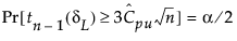
The 100(1 - α)% confidence limits for CPL (denoted by CPLL and CPLU) satisfy the following equations:
 where
where 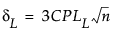
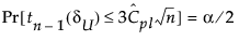 where
where 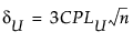
where:
tn-1(δ) has a non-central t-distribution with n - 1 degrees of freedom and noncentrality parameter δ.
 is the estimated value for Cpl.
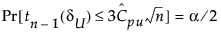
The 100(1 - α)% confidence limits for CPU (denoted by CPUL and CPUU) satisfy the following equations:
 where
where 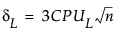
 where
where 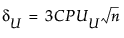
where:
tn-1(δ) has a non-central t-distribution with n - 1 degrees of freedom and noncentrality parameter δ.
 is the estimated value for Cpu.
Capability Indices for Nonnormal Distributions
This section describes how capability indices are calculated for nonnormal distributions. These generalized capability indices are defined as follows:
Cp = 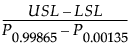
Cpk = 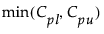
Cpm = 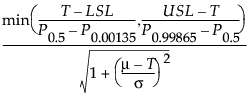
Cpl = 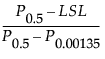
Cpu = 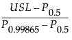
where:
LSL is the lower specification limit.
USL is the upper specification limit.
T is the target value.
Pα is the α*100th percentile of the fitted distribution.
For the calculation of Cpm, μ and σ are estimated using the expected value and square root of the variance of the fitted distribution. For more information about the relationship between the parameters in the Parameter Estimates report and the expected value and variance of the fitted distributions, see Continuous Fit Distributions and Discrete Fit Distributions in Basic Analysis.
Sigma Quality Statistics
The Sigma Quality statistics for each Portion (Below LSL, Above USL, and Total Outside) are calculated as follows:
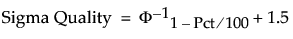
where:
Pct is the value in the Percent column of the report.
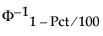 is the (1 - Pct/100)th quantile of a standard normal distribution.
Note: Even though the Percent Below LSL and Percent Above USL sum to the Percent Total Outside value, the Sigma Quality Below LSL and Sigma Quality Above USL values do not sum to the Sigma Quality Total Outside value. This is because calculating Sigma Quality involves finding normal distribution quantiles, and is therefore not additive.
Benchmark Z Statistics
Benchmark Z statistics are available only for capability analyses based on the normal distribution. The Benchmark Z statistics are calculated as follows:
Z Bench = 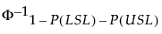
Z LSL =  = 3 * Cpl
Z USL =  = 3 * Cpu
where:
LSL is the lower specification limit.
USL is the upper specification limit.
μ is the sample mean.
σ is the sample standard deviation.
Φ-11 - P(LSL) - P(USL) is the (1 - P(LSL) -P(USL))th quantile of a standard normal distribution.
P(LSL) = Prob(X < LSL) = 1 - Φ(Z LSL).
P(USL) = Prob(X > USL) = 1 - Φ(Z USL).
Φ is the standard normal cumulative distribution function.