Two-Way Split-Plot Experiment
A two-way split-plot (also known as strip-plot or split-block) design consists of two split-plot components. In industry, these designs arise when batches of material or experimental units from one processing stage pass to a second processing stage. To use a two-way split-plot design, you must be able to reorder the units between stages.
After the first processing stage, you must be able to divide the batches into sub-batches. The second-stage processing factors are applied randomly to these sub-batches. For a specific second-stage experimental setting, all of the sub-batches assigned to that setting can be processed simultaneously. Additional factors can be applied to experimental units after the second processing stage.
In contrast to a split-split-plot design, the second-stage factors are not nested within the first-stage factors. After the first stage, the batches are subdivided and formed into new batches. Therefore, both the first- and second-stage factors are applied to whole batches.
Although factors at both stages might be equally hard-to-change, in order to distinguish these factors, JMP denotes the first stage factors as very-hard-to-change and the second-stage factors as hard-to-change. Additional factors applied to experimental units after the second processing stage are considered easy-to-change.
Scenario for a Two-Way Split-Plot Design
This example is based on an experiment to improve the open circuit voltage (OCV) in battery cells (Vivacqua and Bisgaard, 2004). You need to minimize the OCV in order to keep the cells from discharging on their own.
Battery cells move through two stages of processing:
• First stage: A continuous assembly process where batteries are processed in batches of 2000.
• Second stage: A curing process with a 5-day cycle time in a chamber that can accommodate 4000 batteries.
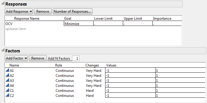
You want to study six two-level continuous factors:
• Four factors (A1, A2, A3, and A4) are applied to the assembly process. You can run 16 trials for the first-stage factors.
• Two factors (C5 and C6) are applied to the curing process. Because curing requires a 5-day cycle time, you can run only 6 cycles (30 days) for the second-stage factors. Using six curing cycles gives you partial replication of the curing settings, enabling you to test for curing effects.
Both the first- and second-stage factors are hard-to-change, suggesting two split-plots. However, the batches of 2,000 batteries from the first-stage experiment can be divided into sub-batches of 500 batteries each. Eight of these sub-batches can be randomly selected and processed simultaneously in the curing chamber.
The experiment has 48 experimental units. Note that the first- and second-stage factors are crossed.
Create the Design
To design a two-way split-plot experiment:
1. Select DOE > Custom Design.
2. Double-click Y under Response Name and type OCV.
3. Under Goal, click Maximize and select Minimize.
4. To add factors manually, follow step 5 through step 10. Or, to load factors from a saved table:
a. Click the Custom Design red triangle and select Load Factors.
b. Open the Battery Factors.jmp sample data table, located in the Design Experiment folder.
c. Proceed to step 11.
5. Type 6 next to Add N Factors.
6. Click Add Factor > Continuous.
7. Rename the factors A1, A2, A3, A4, C1, and C2.
Keep the default Values of -1 and 1 for these factors.
8. For each of the factors A1, A2, A3, and A4, under Changes, click Easy and change it to Very Hard.
To distinguish between the first- and second-stage factors, you designate the Changes for the first-stage factors as Very Hard, and the Changes for the second-stage factors as Hard.
9. For each of the factors C1 and C2, under Changes, click Easy and change it to Hard.
Figure 5.76 Responses and Factors Outlines
10. Click Continue.
11. Select Interactions> 2nd in the Model outline.
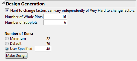
12. In the Design Generation outline, select the option Hard to change factors can vary independently of Very Hard to change factors.
See Figure 5.77. Checking this option creates a two-way split-plot design. If this option is not checked, the design is treated as a split-split-plot design, with nesting of factors at the two levels.
13. Type 16 as the Number of Whole Plots.
This is the number of trials that you can run for the first-stage factors.
14. Type 6 as the Number of Subplots.
This is the number of trials that you can run for the second-stage factors.
15. Under Number of Runs, type 48 next to User Specified.
This is the total number of experimental units.
Figure 5.77 Design Generation Outline
Note: Setting the Random Seed in step 16 and Number of Starts in step 17 reproduces the exact results shown in this example. In constructing a design on your own, these steps are not necessary.
16. (Optional) Click the Custom Design red triangle, select Set Random Seed, type 1866762673, and click OK.
17. (Optional) Click the Custom Design red triangle, select Number of Starts, type 21, and click OK.
18. Click Make Design.
19. Click Make Table.
Figure 5.78 Partial View of Design Table
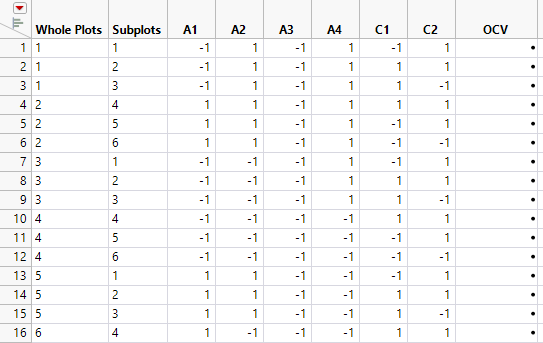
The design table shows 16 levels for Whole Plots. For each level of Whole Plots, the settings of the four assembly factors are constant. From each level of Whole Plots, three batches of 500 batteries (Subplots) are randomly assigned to settings of the curing factors. Two sets of curing conditions are replicated (C1 = -1, C2 = 1 and C1 = 1, C2 = 1). To see this, select columns C1 and C2, right-click in the header area, and select Sort > Ascending.
Analyze the Results
The Battery Data.jmp sample data table contains experimental results for the design that you generated.
1. Select Help > Sample Data Library and open Design Experiment/Battery Data.jmp.
2. In the Table panel, click the green triangle next to the Model script.
Notice the following in the Fit Model window:
– The factor Whole Plots has the Attribute called Random Effects (&Random). This specifies that the levels of Whole Plots are random realizations. They have an associated error term.
– The factor Subplots also has the Random Effects Attribute (&Random).
– The analysis Method is REML (Recommended). This method is specified precisely because the model contains random effects. For more information about REML models, see Restricted Maximum Likelihood (REML) Method in Fitting Linear Models.
Tip: In the Fit Model window, JMP Pro users can change the Personality to Mixed Model.
3. Check the option to Keep dialog open.
4. Click Run.
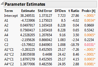
Figure 5.79 Report for Full Model
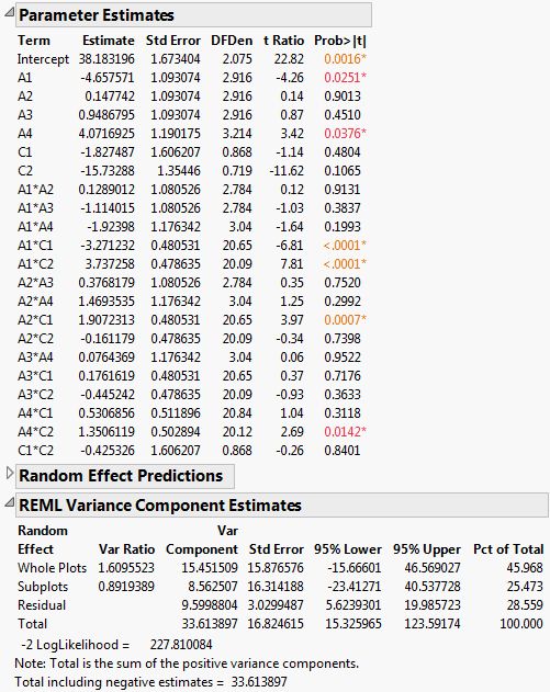
The Parameter Estimates report indicates that four two-way interactions, A1*C1, A1*C2, A2*C1, and A4*C2, and two main effects, A1 and A4, are significant at the 0.05 level.
5. In the Table panel of Battery Data.jmp, click the green triangle next to the Reduced Model 1 script.
The script opens a Fit Model window where insignificant interactions have been removed. The remaining effects are all main effects and the four two-way interactions A1*C1, A1*C2, A2*C1, and A4*C2. You are reducing the model in a conservative fashion.
6. Click Run.
Figure 5.80 Report for Preliminary Reduced Model
Notice that the main effect C2 is now significant at the 0.05 level (Prob>|t| = 0.0331)
7. In the Fit Model window, remove A3.
The main effect A3 is the only main effect that is not significant and not involved in a two-way interaction.
8. Click Run.
Figure 5.81 Report for Reduced Model
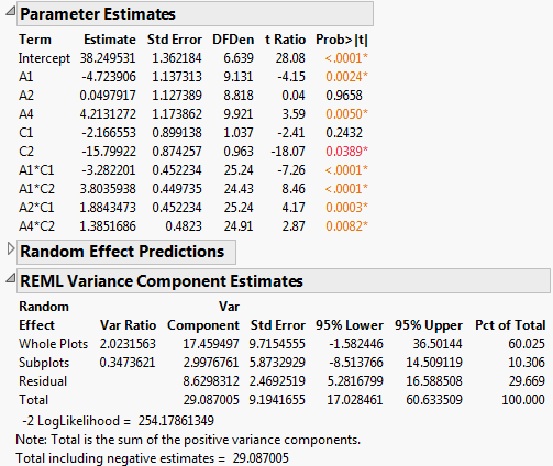
The REML Variance Component Estimates report shows that the variance component associated with Whole Plots is about six times as large as the variance component for Subplots. This suggests that the assembly process is more variable than the curing process. Also, the within (Residual) error is larger than that for Subplots. Efforts to reduce variation should focus on the assembly process and on battery-to-battery differences.
9. Click the Response OCV red triangle and select Factor Profiling > Profiler.
10. Click the Prediction Profiler red triangle and select Optimization and Desirability > Maximize Desirability.
Figure 5.82 Prediction Profiler with Settings That Minimize OCV
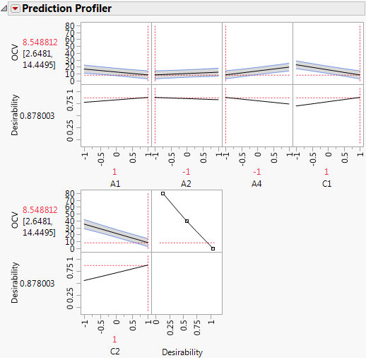
The profiler shows the five factors identified as active and settings that minimize OCV.