Weibull Loss Function Using the Nonlinear Platform
In this example, models are fit to the survival time using the Weibull, lognormal, and exponential distributions. Model fits include a simple survival model containing only two effects, a more complex model with all the effects, and the creation of dummy variables for the discrete effect Cell Type to be included in the full model.
Nonlinear model fitting is often sensitive to the initial values that you give to the model parameters. In this example, one way to find reasonable initial values is to first use the Nonlinear platform to fit only the linear model. When the model converges, the solution values for the parameters become the initial parameter values for the nonlinear model.
1. Select Help > Sample Data Library and open VA Lung Cancer.jmp.
The first model and all the loss functions have already been created as formulas in the data table. The Model column has the following formula:
Log(:Time) - (b0 + b1 * Age + b2 * Diag Time)
2. Select Analyze > Specialized Modeling > Nonlinear.
3. Select Model and click X, Predictor Formula.
4. Click OK.
5. Click Go.
Figure 14.16 Initial Parameter Values in the Nonlinear Fit Control Panel
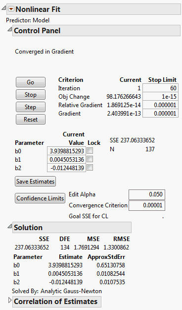
The report computes the least squares parameter estimates for this model.
6. Click Save Estimates.
The parameter estimates in the column formulas are set to those estimated by this initial nonlinear fitting process.
The Weibull column contains the Weibull formula, explained in Weibull Loss Function.
To continue with the fitting process:
7. Select Analyze > Specialized Modeling > Nonlinear again.
8. Select Model and click X, Predictor Formula.
9. Select Weibull loss and click Loss.
10. Click OK.
The Nonlinear Fit Control Panel on the left in Figure 14.17 appears. There is now the additional parameter called sigma in the loss function. Because it is in the denominator of a fraction, a starting value of 1 is reasonable for sigma. When using any loss function other than the default, the Loss is Neg LogLikelihood box on the Control Panel is checked by default.
11. Click Go.
The fitting process converges as shown on the right in Figure 14.17.
Figure 14.17 Nonlinear Model with Custom Loss Function
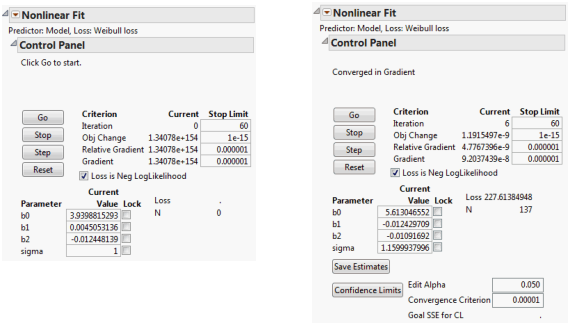
The fitting process estimates the parameters by maximizing the negative log of the Weibull likelihood function.
12. (Optional) Click Confidence Limits to show lower and upper 95% confidence limits for the parameters in the Solution table.
Figure 14.18 Solution Report
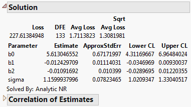
Note: Because the confidence limits are profile likelihood confidence intervals instead of the standard asymptotic confidence intervals, they can take time to compute.
You can also run the model with the predefined exponential and lognormal loss functions. Before you fit another model, reset the parameter estimates to the least squares estimates, as they might not converge otherwise. To reset the parameter estimates:
13. (Optional) Click the Nonlinear Fit red triangle and select Revert to Original Parameters.