Analyze the Data
Now you are ready to run your experiment, gather the Rating data, and insert the results in the Rating column of your Custom Design table.
1. Select Help > Sample Data Library and open Design Experiment/Wine Data.jmp.
The Wine Data.jmp table is exactly the same as the Custom Design table shown in Figure 4.9, except that it contains your recorded experimental results.
2. In the Table panel, click the green triangle next to the Model script.
Figure 4.10 Fit Model Dialog for Wine Experiment
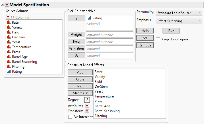
Notice that Rater, the blocking factor, is added as a fixed effect, rather than as a random block effect. This is appropriate because the five raters were specifically chosen and are not a random sample from a larger population.
3. Click Run.
Interpret the Full Model Results
The results are shown below.
Figure 4.11 Partial Model Fit Results
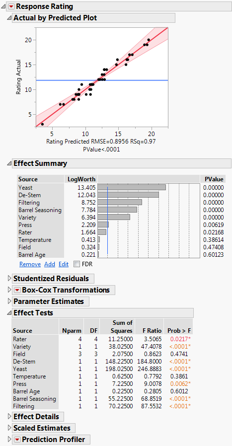
Note the following:
• The Actual by Predicted Plot shows no obvious evidence of lack of fit.
• The model is significant, as indicated by the Actual by Predicted Plot and by the p-value beneath it.
• The Effect Tests report indicates that seven of the model terms are significant at the 0.05 level. Field, Temperature, and Barrel Age are not significant.
• The Effect Summary report lists these effects in decreasing order of significance. Larger LogWorth values correspond to smaller PValues and greater significance.
Reduce the Model
Reduce the model by removing the effects that you identified as inactive:
1. In the Effect Summary report, press the Control key and hold it as you select Temperature, Field, and Barrel Age.
2. Click Remove.
The report updates to show the model fit with these three effects removed.
Interpret the Reduced Model Results
The Actual by Predicted Plot for the reduced model shows no lack of fit issues. The Effect Summary and the Effect Test report show that the remaining seven terms are significant at the 0.05 level.
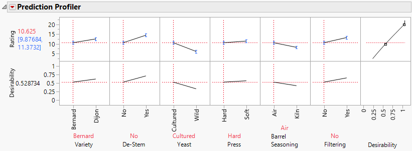
Figure 4.12 shows the Prediction Profiler. Recall that you specified a response goal of Maximize, with lower and upper limits of 0 and 20. Setting these limits caused a Response Limits column property to be saved to the Rating column in the Custom Design table. The Prediction Profiler uses the Response Limits information to construct a Desirability function, which appears in the right-most plot in the top row in Figure 4.12. The bottom row displays Desirability traces.
The first six plots in the top row show traces of the predicted model. For each factor, the line in the plot shows how Rating varies when all other factors are set at the values defined by the red dashed vertical lines. By default, the profiler appears with categorical factors set at their low settings. By varying the settings for the factors, you can see how the predicted Rating for wines changes. Notice that a confidence interval is given for the mean predicted Rating.
Observe that Rater is not included among the factors shown in the profiler. This is because Rater is a block variable. You included Rater to explain variation, but Rater is not of direct interest in terms of optimizing process factor settings. The predicted Rating for a wine with the given settings is the average of the predicted ratings for that wine by all raters.
Figure 4.12 Profiler for Reduced Model
Optimize Factor Settings
You would like to identify settings that maximize Rating across raters.
1. Click the Prediction Profiler red triangle and select Optimization and Desirability > Maximize Desirability.
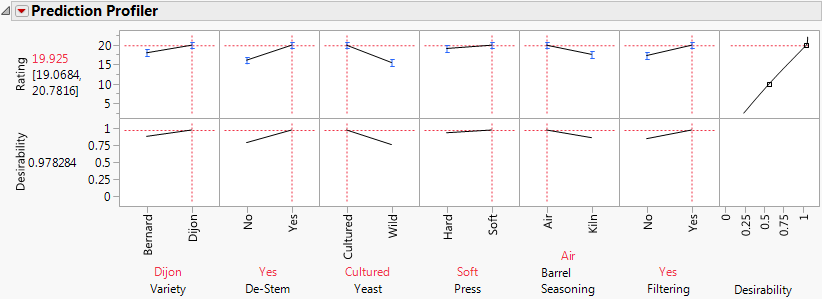
The red dashed vertical lines in the Prediction Profiler update to show optimal settings for each factor. The optimal settings result in a predicted rating of 19.925. In general, there can be different sets of factor settings that result in the same optimal value.
Figure 4.13 Prediction Profiler with Factor Settings Optimized
2. To see predicted ratings for all runs, save the Prediction Formula. Click the Response Rating red triangle and select Save Columns > Prediction Formula.
A column called Pred Formula Rating is added to the data table. Note that one of the runs, row 33, was given the maximum rating of 20 by Rater 5. The predicted rating for that run by Rater 5 is 19.550. But the row 33 trial was run at the optimal settings. The predicted value of 19.925 given for these settings in the Prediction Profiler is obtained by averaging the predicted ratings for that run over all five raters.
Lock a Factor Level
When you maximized desirability, you learned that the optimal rating is achieved with the Dijon variety of grapes (Figure 4.13). Your manager points out that it would be cost-prohibitive to replant the fields that are growing Bernard grapes with young Dijon vines. Therefore, you need to find optimal process settings and the predicted rating for Bernard grapes.
1. In the Variety plot of the Prediction Profiler, drag the red dashed vertical line to Bernard.
2. Press Control and click in one of the Variety plots.
The Factor Settings window appears.
3. Select Lock Factor Setting and click OK.
4. Click the Prediction Profiler red triangle and select Optimization and Desirability > Maximize Desirability.
Figure 4.14 Prediction Profiler with Optimal Settings for Bernard Variety
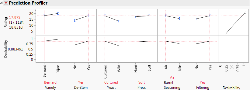
The optimal settings are unchanged because the model contains no interaction terms. The predicted rating at these settings is 17.975.
Profiler with Rater
If you want to see the Profiler traces for the levels of Rater, perform the following steps:
1. Click the Prediction Profiler red triangle and select Reset Factor Grid.
A Factor Settings window appears with columns for all of the factors, including Rater. The box under Rater and next to Show is not checked. This indicates that Rater is not shown in the Prediction Profiler.
2. Check the box under Rater in the row corresponding to Show.
3. Deselect the box under Rater in the row corresponding to Lock Factor Setting.
4. Click OK.
The Profiler updates to show a plot for Rater.
5. Click in either plot above Rater.
Figure 4.15 Profiler for Reduced Model Showing Rater
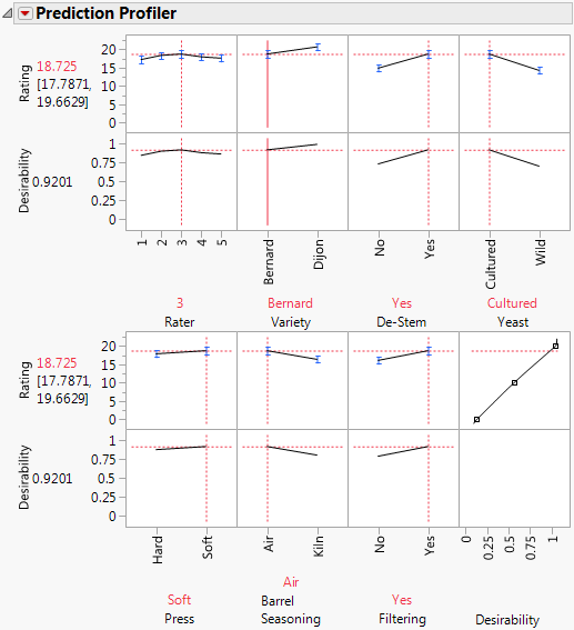
A dashed vertical red line appears. Drag this line to see the traces for each of the raters. Keep in mind that Variety is still locked at Bernard. To unlock Variety, press Control and click in one of the Variety plots. In the Factor Settings window that appears, deselect Lock Factor Setting.
Summary
In your wine tasting experiment, using only 40 runs, you have identified six (out of nine) factors that have an effect on ratings for Pinot Noir grapes. You found that you could achieve a predicted rating of 19.925 (out of a possible 20) at the optimal settings for those factors. You also identified optimal settings for both varieties of grapes.
In this section, you constructed a design using the outlines in the Custom Design window. The next section explains each outline and the design steps in more detail.