Principal Components Report Options
The Principal Components red triangle menu contains the following options:
Note: Some of the options are not available for the Wide or Sparse estimation methods.
Principal Components
(Not available for the Wide or Sparse estimation methods.) Enables you to create the principal components based on Correlations, Covariances, or Unscaled.
Correlations
(Not available for the Wide or Sparse estimation methods.) The matrix of correlations between the variables.
Note: The values on the diagonals are 1.0.
Covariance Matrix
(Not available for the Wide or Sparse estimation methods.) Shows or hides the covariances of the variables.
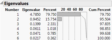
Eigenvalues
Lists the eigenvalue that corresponds to each principal component in order from largest to smallest. The eigenvalues represent a partition of the total variation in the multivariate sample.
The scaling of the eigenvalues depends on which matrix you select for extraction of principal components:
– For the on Correlations option, the eigenvalues are scaled to sum to the number of variables.
– For the on Covariances options, the eigenvalues are not scaled.
– For the on Unscaled option, the eigenvalues are divided by the total number of observations.
If you select the Bartlett Test option from the red triangle menu, hypothesis tests (Figure 4.6) are given for each eigenvalue (Jackson 2003).
Figure 4.5 Eigenvalues
Eigenvectors
Shows or hides a table of the eigenvectors for each of the principal components, in order, from left to right. Using these coefficients to form a linear combination of the original variables produces the principal component variables. Following the standard convention, eigenvectors have norm 1.
Note: The number of eigenvectors shown is equal to the rank of the correlation matrix, or, if the Sparse method is selected, the number of components specified on the launch window.
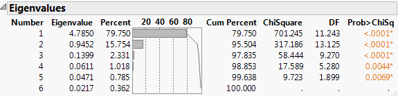
Bartlett Test
(Not available for the Wide or Sparse estimation methods.) Shows or hides the results of the homogeneity test (appended to the Eigenvalues table). The test determines whether the eigenvalues have the same variance by calculating the Chi-square, degrees of freedom (DF), and the p-value (prob > ChiSq) for the test. See Bartlett (1937, 1954).
Figure 4.6 Bartlett Test
Loading Matrix
Shows or hides a table of the loadings for each component. These values are graphed in the loading plot. The degree of transparency for the table values indicates the distance of the absolute loading value from zero. Absolute loading values that are closer to zero are more transparent than absolute loading values that are farther from zero.
If you specify a supplementary variable, an additional table of coordinates is shown for each supplementary continuous variable and each level of supplementary categorical variable. These values are graphed in the loading plot for continuous supplementary variables.
The scaling of the loadings and coordinates depends on which matrix you select for extraction of principal components:
– For the on Correlations option, the ith column of loadings is the ith eigenvector multiplied by the square root of the ith eigenvalue. The i,jth loading is the correlation between the ith variable and the jth principal component.
– For the on Covariances option, the jth entry in the ith column of loadings is the ith eigenvector multiplied by the square root of the ith eigenvalue and divided by the standard deviation of the jth variable. The i,jth loading is the correlation between the ith variable and the jth principal component.
– For the on Unscaled option, the jth entry in the ith column of loadings is the ith eigenvector multiplied by the square root of the ith eigenvalue and divided by the standard error of the jth variable. The standard error of the jth variable is the jth diagonal entry of the sum of squares and cross products matrix divided by the number of rows (X′X/n).
Note: When you are analyzing the unscaled data, the i,jth loading is not the correlation between the ith variable and the jth principal component.
Formatted Loading Matrix
Shows or hides a table of the loadings for each component. The table is sorted in order of decreasing loadings on the first principal component. Therefore, the variables are listed in the order of decreasing loadings on the first component.
Figure 4.7 Formatted Loading Matrix
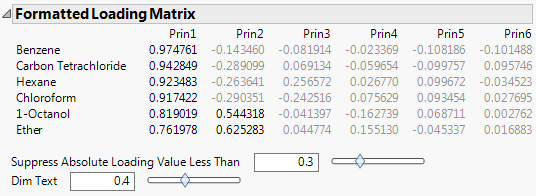
Suppress Absolute Loading Value Less Than
The value that determines which loadings are unavailable in the Formatted Loading Matrix report. You can use the text box or the slider to dim the loadings whose absolute values fall below the selected value.
Dim Text
The transparency of the dimmed values in the Formatted Loading Matrix report. You can use the text box or the slider to set the degree of transparency for the dimmed loadings. The degree of transparency ranges from 0 to 1, where lower values are more transparent than higher values. For example, setting the transparency to 0 completely removes the unavailable loadings from the matrix, while the loadings are still available when you set the transparency to 1.
Squared Cosines of Variables
Shows or hides a table that contains the squared cosines of variables. If you specify a supplementary variable, an additional table of squared cosines of supplementary variables is shown. The sum of the squared cosine values across principal components is equal to one for each variable. The squared cosines enable you to see how well the variables are represented by the principal components. You can also determine how many principal components are necessary to represent certain variables. This option also shows a plot of the squared cosines for the first three principal components.
Note: If the Sparse estimation method is used and the number of components selected is less than three, only the specified number of components are displayed in the plot.
Partial Contribution of Variables
Shows or hides a table that contains the partial contributions of variables. The partial contributions enable you to see the percentage that each variable contributes to each principal component. This option also shows a plot of the partial contributions for the first three principal components.
Note: If the Sparse estimation method is used and the number of components selected is less than three, only the specified number of components are displayed in the plot.
Summary Plots
Shows or hides the summary information produced in the default report. This summary information includes a plot of the eigenvalues, a score plot, and a loading plot. By default, the report shows the score and loading plots for the first two principal components. There are options in the report to specify which principal components to plot. See Principal Components Report.
Tip: Select the tips of arrows in the loading plot to select the corresponding columns in the data table. Hold down Ctrl and click an arrow tip to deselect the column.
Biplot
Shows or hides a plot that overlays the score plot and the loading plot for the specified number of components.
Figure 4.8 Biplot
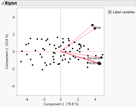
Note: The score plot markers are dots and the loading plot markers are diamonds.
Scatterplot Matrix
Shows or hides a matrix of score and loading plots for a specified number of principal components. The scatterplot matrix arranges both the score plots and the loading plots in one space. The score plots have a yellow shaded background. The loading plots have a blue shaded background.
Figure 4.9 Scatterplot Matrix
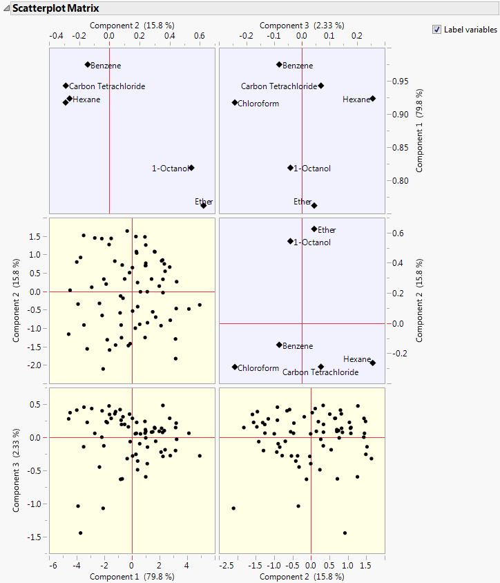
Note: The loading plot matrix displayed in the Scatterplot Matrix is the transpose of the loading plot matrix that you obtain when you select the Loading Plot option.
Scree Plot
Shows or hides a graph of the eigenvalue for each component. This scree plot helps in visualizing the dimensionality of the data space.
Score Plot
Shows or hides a matrix of scatterplots of the scores for pairs of principal components for the specified number of components. This plot is shown in Figure 4.4 (left-most plot).
Loading Plot
Shows or hides a matrix of two-dimensional representations of factor loadings for the specified number of components. The loading plot labels variables if the number of variables is 30 or fewer. If there are more than 30 variables, the labels are off by default. This information is shown in Figure 4.4 (right-most plot).
Tip: Select the tips of arrows in the loading plot to select the corresponding columns in the data table. Hold down Ctrl and click an arrow tip to deselect the column.
Score Plot with Imputation
(Not available for the Wide or Sparse estimation methods.) Imputes any missing values and creates a score plot. This option is available only if there are missing values.
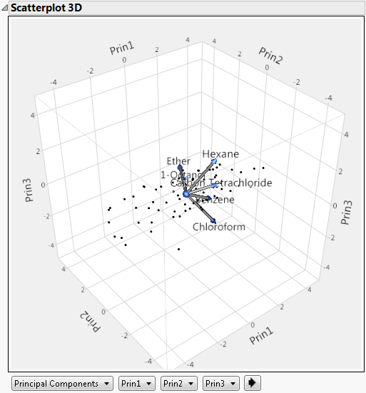
3D Score Plot
(Not available for the Wide or Sparse estimation methods.) Shows or hides a 3D scatterplot of any three principal component scores. When you first invoke the command, the first three principal components are presented.
Figure 4.10 Scatterplot 3D Score Plot
Plot Source
The source of the data points in the plot. The available options are Principal Components, Rotated Principal Components, and Data Columns.
Axis Controls
The contents of each axis. If the Principal Components option or the Rotated Components option is selected, the options for the Axis Controls are principal components. If the Data Columns option is selected, the options are variables from the analysis.
Cycle Button![]()
Cycles through all axis content possibilities.
The variables show as rays in the plot. These rays, called biplot rays, approximate the variables as a function of the principal components on the axes. If there are only two or three variables, the rays represent the variables exactly. The ray corresponds to the principal component loadings.
Score Ellipses
Shows or hides ellipses on the summary score plot for each pair of principal components. The ellipses are constructed as either confidence ellipses based on the alpha level or a control limit ellipses based on how far the observations are from the center. By default, the ellipses are 95% confidence ellipses.
Score Ellipse Coverage
Displays a submenu that enables you to change how the score ellipses are constructed. Specify the score ellipses by confidence level or the distance from the center in terms of k-sigma. The relationship between the confidence level, p, and k-sigma is p = 1 - exp(-k2/2).
Display Options
Arrow Lines
Enables you to show or hide arrows on all plots that can display arrows. Arrows are shown if the number of variables is 1000 or fewer. If there are more than 1000 variables, the arrows are off by default.
Show Supplementary Variable
(Available only if you specify a supplementary variable.) Shows or hides the arrow lines for continuous supplementary variables or label markers for categorical supplementary variables in the biplot, score plot, and loading plots.
Outlier Analysis
Shows or hides the Outlier Analysis report, which enables you to detect outliers in the data through T2 and contribution statistics. See Outlier Analysis.
Factor Analysis
(Not available for the Wide or Sparse estimation methods.) Performs factor analysis-style rotations of the principal components, or factor analysis. See Factor Analysis.
 Cluster Variables
(Not available for the Wide or Sparse estimation methods.) Performs a cluster analysis on the variables by dividing the variables into non-overlapping clusters. Variable clustering provides a method for grouping similar variables into representative groups. Each cluster can then be represented by a single component or variable. The component is a linear combination of all variables in the cluster. Alternatively, the cluster can be represented by the variable identified to be the most representative member in the cluster. See Cluster Variables.
Note: Cluster Variables uses correlation matrices for all calculations, even when you select the on Covariance or on Unscaled options.
Save Principal Components
Saves the number of principal components that you specify to the data table with a formula for computing each component. The formula cannot evaluate rows with missing values.
The calculation for the principal components depends on which matrix you select for extraction of principal components:
– For the on Correlations option, the ith principal component is a linear combination of the centered and scaled observations using the entries of the ith eigenvector as coefficients.
– For the on Covariances options, the ith principal component is a linear combination of the centered observations using the entries of the ith eigenvector as coefficients.
– For the on Unscaled option, the ith principal component is a linear combination of the raw observations using the entries of the ith eigenvector as coefficients.
Note: If the specified number of components exceeds the rank of the correlation matrix, then the number of components saved is set to the rank of the correlation matrix.
Save Predicteds
Saves the predicted variables with a specified number of principal components to new columns in the data table.
Save DModX
Saves the observation distance to the principal components model (DModX) to a new column in the data table. Larger DModX values indicate mild to moderate outliers in the data. See DModX Calculation.
Save Individual Squared Cosines
Saves the individual squared cosines to new columns in the data table.
Save Individual Partial Contributions
Saves the individual partial contributions to new columns in the data table.
Save Rotated Components
(Not available for the Wide or Sparse estimation methods.) Saves the rotated components to the data table, with a formula for computing the components. This option is available only after the Factor Analysis option is used. The formula cannot evaluate rows with missing values.
Save Principal Components with Imputation
(Not available for the Wide or Sparse estimation methods.) Imputes missing values, and saves the principal components to the data table. The column contains a formula for doing the imputation and computing the principal components. This option is available only if there are missing values.
Save Rotated Components with Imputation
(Not available for the Wide or Sparse estimation methods.) Imputes missing values and saves the rotated components to the data table. The column contains a formula for doing the imputation and computing the rotated components. This option is available only after the Factor Analysis option is used and if there are missing values.
 Publish Components Formulas
Creates a specified number of principal component formulas and saves them as formula column scripts in the Formula Depot platform. If a Formula Depot report is not open, this option creates a Formula Depot report. See Formula Depot in Predictive and Specialized Modeling.
 Publish DModX Formula
Saves the DModX formula based on a specified number of principal components as a formula column script in the Formula Depot platform. If a Formula Depot report is not open, this option creates a Formula Depot report. See Formula Depot in Predictive and Specialized Modeling.
See Local Data Filter, Redo Menus, and Save Script Menus in Using JMP for more information about the following options:
Local Data Filter
Shows or hides the local data filter that enables you to filter the data used in a specific report.
Redo
Contains options that enable you to repeat or relaunch the analysis. In platforms that support the feature, the Automatic Recalc option immediately reflects the changes that you make to the data table in the corresponding report window.
Save Script
Contains options that enable you to save a script that reproduces the report to several destinations.
Save By-Group Script
Contains options that enable you to save a script that reproduces the platform report for all levels of a By variable to several destinations. Available only when a By variable is specified in the launch window.