Analyze the Data
The Custom Design platform facilitates the task of data analysis by saving a Model script to the design table that it creates (Figure 3.10). Run this script after you conduct your experiment and enter your data. The script opens a Fit Model window containing the effects that you specified in the Model outline of the Custom Design window.
Fit the Model
1. Select Help > Sample Data Library and open Design Experiment/Coffee Data.jmp.
In the Table panel, notice the Model script created by Custom Design.
2. Click the green triangle next to the Model script.
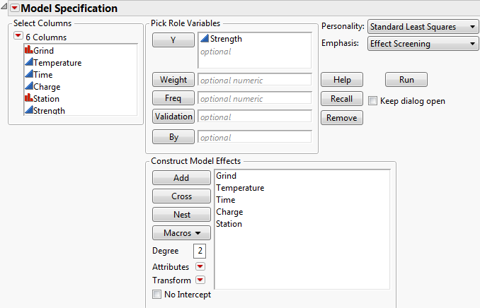
The Model Specification window shows the effects that you specified in the Model outline.
Figure 3.12 Model Specification Window
3. Select the Keep dialog open option.
4. Click Run.
Analyze the Model
The Effect Summary and Actual by Predicted Plot reports give high-level information about the model.
Figure 3.13 Effect Summary and Actual by Predicted Plot for Full Model
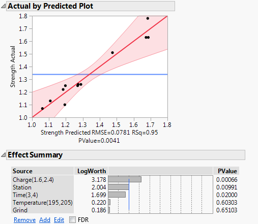
Note the following:
• The Actual by Predicted Plot shows no evidence of lack of fit.
• The model is significant, as indicated by the Actual by Predicted Plot. The notation P = 0.0041, shown below the plot, gives the significance level of the overall model test.
• The Effect Summary report shows that Charge, Station, and Time are significant at the 0.05 level.
• The Effect Summary report also shows that Temperature and Grind are not significant.
Reduce the Model
Because Temperature and Grind appear not to be active, they contribute random noise to the model. Refit the model without these effects to obtain more precise estimates of the model parameters associated with the active effects.
1. In the Model Specification window, select Temperature and Grind in the Construct Model Effects list.
2. Click Remove.
3. Confirm that the model Emphasis is set to Effect Screening.
The Effect Screening emphasis presents reports (such as the Prediction Profiler) that are useful for analyzing experimental designs.
4. Click Run.
Figure 3.14 Partial Output for the Reduced Model
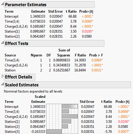
Note the following:
• The Effect Tests report shows that all three effects remain significant.
• The Scaled Estimates report further indicates that the Station[1]and Station[3] means differ significantly from the average response of Strength.
• Note that the Estimates that appear in the Parameter Estimates report are identical to their counterparts in the Scaled Estimates report. This is because the effects are coded. See Coding in the Column Properties section.
• The estimate of the Station[3] effect only appears in the Scaled Estimates report, where nominal factors are expanded to show estimates for all their levels.
• The Parameter Estimates report gives estimates for the model coefficients where the model is specified in terms of the coded effects.
Explore the Model
The Prediction Profiler appears at the bottom of the report.
Figure 3.15 Prediction Profiler
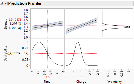
Recall that, in designing your experiment, you set a response Goal of Match Target with limits of 1.2 and 1.4. JMP uses this information to construct a desirability function to reflect your specifications. See Factors.
Note the following in Figure 3.15:
• The first two plots in the top row of the graph show how Strength varies for one of the factors, given the setting of the other factor. For example, when Charge is 2, the line in the plot for Time shows how predicted Strength changes with Time.
• The values to the left of the top row of plots give the Predicted Strength (in red) and a confidence interval for the mean Strength for the selected factor settings.
• The right-most plot in the top row shows the desirability function for Strength. The desirability function indicates that the target of 1.3 is most desirable. Desirability decreases as you move away from that target. Desirability is close to 0 at the limits of 1.2 and 1.4.
• The plots in the bottom row show the desirability trace for each factor at the setting of the other factor.
• The value to the left of the bottom row of plots gives the Desirability of the response value for the selected factor settings.
Explore various factor settings by dragging the red dashed vertical lines in the columns for Time and Charge. Since there are no interactions in the model, the profiler indicates that increasing Charge increases Strength. Also, Strength seems to be more sensitive to changes in Charge than to changes in Time.
Since Station is a blocking factor, it does not appear in the Prediction Profiler. However, you might like to see how predicted Strength varies by Station. To include Station in the Prediction Profiler, follow these steps:
1. Click the Prediction Profiler red triangle and select Reset Factor Grid.
A Factor Settings window appears with columns for Time, Charge, and Station. Under Station, notice that the box corresponding to Show is not selected. This indicates that Station is not shown in the Prediction Profiler.
2. Select the box under Station in the row corresponding to Show.
3. Deselect the box under Station in the row corresponding to Lock Factor Setting.
Figure 3.16 Factor Settings Window
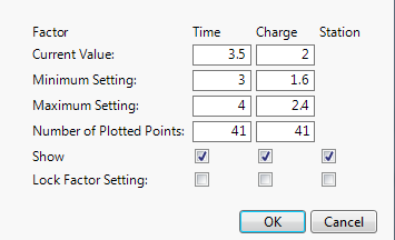
4. Click OK.
Plots for Station appear in the Prediction Profiler.
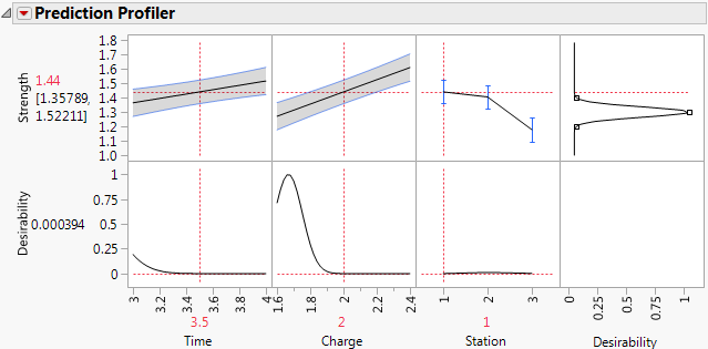
5. Click in either plot above Station to insert a dashed red vertical line.
6. Move the dashed red vertical line to Station 1.
Figure 3.17 Prediction Profiler Showing Results for Station 1
7. Move the dashed red vertical line to Station 3.
Figure 3.18 Prediction Profiler Showing Results for Station 3
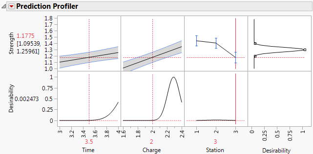
The predicted Strength in the center of the design region for Station 1 is 1.44. For Station 3, the predicted Strength is about 1.18. The magnitude of the difference indicates that you need to address Station variability. Better control of Station variation should lead to more consistent Strength. Once Station consistency is achieved, you can determine common optimal settings for Time and Charge.
The process that you used to construct the design for the coffee experiment followed the steps in the DOE workflow. The next section describes the DOE workflow in more detail.