Guidelines for the Analysis of Deterministic Data
It is important to remember that deterministic data have no random component. The same input values generate the same output. As a result, p-values from fitted statistical models do not have their usual meanings. A large F statistic (low p-value) is an indication of an effect due to a model term. However, you cannot construct valid confidence intervals for effects or model predictions.
Residuals from a model fit to deterministic data are not a measure of noise. Instead, residuals are a measure of the model bias. Bias is the difference between the true value and the predicted value. Distinct patterns in the residuals indicate that additional terms should be considered for the model in order to reduce bias.
Analysis of the Borehole Sphere-Packing Design
Often, the true model is not available in a simple analytical form. As a result, the prediction bias is known only at observed data points. However, in this example, the functional form of the true model is known. In the Borehole Sphere Packing.jmp data table, the true model column contains the formula of the known function. This formula enables you to profile the prediction bias over the factor input region.
1. Select Help > Sample Data Library and open Design Experiment/Borehole Sphere Packing.jmp.
2. Click the green triangle next to the Model (GP from DOE) script.
Use the Gaussian Process Model report to explore the relationships between the factors and the outcome Y.
3. Click the red triangle next to Gaussian Process Model of Y and select Save Prediction Formula.
4. Go back to the Borehole Sphere Packing.jmp data table.
5. In the data grid, select the column headings for true model and Y Prediction Formula.
6. Right-click and select New Formula Column > Combine > Difference.
This creates a new column containing the bias.
7. From the Borehole Sphere Packing.jmp data table, select Graph > Profiler.
8. Select true model-Y Prediction Formula and click Y, Prediction Formula
9. Select Expand Intermediate Formulas.
This option shows the bias as a function of the eight design factors.
Figure 21.30 Profiler Dialog for Borehole Sphere-Packing Data
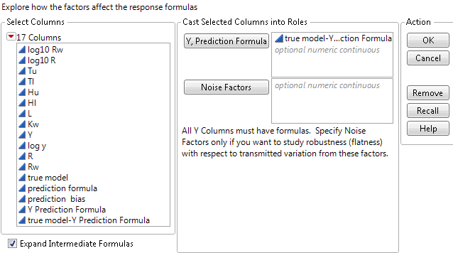
10. Click OK.
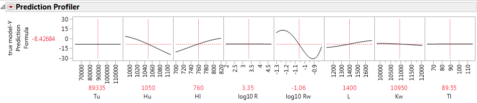
The profiler defaults to the center of the design region. If there were no bias, all profile traces would be constant between the value ranges of each factor. In this example, the variables logRw, Hu, and Hl show the largest effects on the bias.
Figure 21.31 Profiler for Bias of the Borehole GP Model with Y Axis Set at -30 to 30
You can use the profiler to explore the range of the prediction bias over the entire domain. To find points of minimum and maximum bias, select Optimization and Desirability > Desirability Functions from the Prediction Profiler red triangle menu. See Desirability Profiling and Optimization in Profilers. To evaluate the prediction bias over the design points, select Analyze > Distribution to see a distribution analysis.
Figure 21.32 Distribution of the Prediction Bias
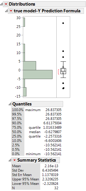
Keep in mind that, in this example, the true model is known. In many applications, the response at any factor setting is unknown. The prediction bias over the experimental data can underestimate the bias throughout the design domain.