Example of a Quadratic Ordinal Logistic Model
The Ordinal Logistic Personality can fit a quadratic surface to optimize the probabilities of higher or lower levels of an ordinal response.
In this example, a microwave popcorn manufacturer wants to find out how much salt consumers like in their popcorn. To do this, the manufacturer looks for the maximum probability of a favorable response as a function of how much salt is added to the popcorn package. In this experiment, the salt amounts are controlled at 0, 1, 2, and 3 teaspoons. Respondents rate the taste on a scale of 1 (low) to 5 (high). The optimal amount of salt is the amount that maximizes the probability of more favorable responses. The ten observations for each of the salt levels are shown in Table 11.2.
|
Salt Amount |
Salt Rating Responses |
|---|---|
|
no salt |
1, 3, 2, 4, 2, 2, 1, 4, 3, 4 |
|
1 tsp. |
4, 5, 3, 4, 5, 4, 5, 5, 4, 5 |
|
2 tsp. |
4, 3, 5, 1, 4, 2, 5, 4, 3, 2 |
|
3 tsp. |
3, 1, 2, 3, 1, 2, 1, 2, 1, 2 |
1. Select Help > Sample Data Library and open Salt in Popcorn.jmp.
2. Select Analyze > Fit Model.
3. Select Taste Test from the Select Columns list and click Y.
4. Select Salt from the Select Columns list and click Macros > Response Surface.
5. Click Run.
6. Click the disclosure icon next to Response Surface to open the report.
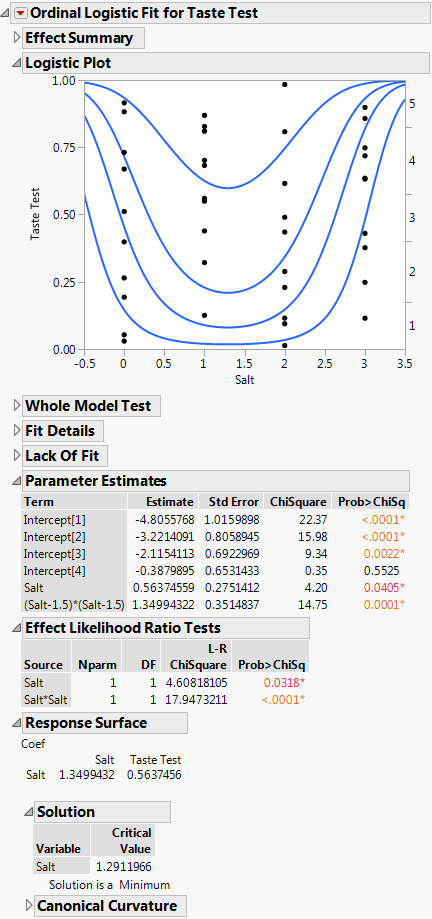
Figure 11.11 Ordinal Logistic Fit for Salt in Popcorn.jmp
The report shows how the quadratic model fits the response probabilities. The curves, instead of being shifted logistic curves, become stacked U-shaped curves where each curve achieves its minimum at the same point. The critical value is at Mean(X) – 0.5 * (b1/b2) where b1 is the linear coefficient and b2 is the quadratic coefficient. This formula is for centered X. From the Parameter Estimates table, you can compute that the optimal amount of salt is 1.5 - 0.5 * (0.5637/1.3499) = 1.29 teaspoons.
The vertical distance at a specific amount of salt between each curve measures the probability of each of the five response levels for the specific amount of salt. The probability for the highest response level is the distance from the top curve to the top of the plot rectangle. This distance reaches a maximum when the amount of salt is about 1.3 teaspoons. All curves share the same critical point.
The parameter estimates for Salt and Salt*Salt are the coefficients used to find the critical value. Although the critical value appears on the logistic plot as a minimum, it is a maximum in the sense of maximizing the probability of the highest response. The Solution portion of the report is shown under Response Surface in Figure 11.11, where 1.29 is shown under Critical Value.
