Willingness to Pay
The term willingness to pay refers to the price that a customer is willing to pay for new features, calculated to match a customer’s utility for baseline features. For example, suppose that a customer is willing to pay $1,000 for a computer with a 40 GB hard drive. Willingness to Pay for an 80 GB hard drive is calculated by setting the Hard drive feature to 80 GB and then solving for the price that delivers the same utility as the $1000 40 GB hard drive.
Willingness to Pay Launch Window Options
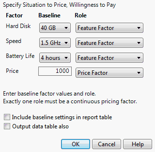
When you select the Willingness to Pay option, the Willingness to Pay launch window is shown. The launch window in Figure 4.20 is obtained by selecting the Willingness to Pay option in the report that results from running the Choice data table script in Laptop Profile.jmp.
Factor
The variables from the analysis. These can be product features or subject-specific attributes.
Baseline
The baseline setting for each factor. If the factor is categorical, select the baseline value from a list. If the factor is numeric, enter the baseline value.
Role
The type of factor.
Feature Factor
A product or service feature from the experiment that you want to price.
Price Factor
A price factor in the experiment. The price factor must be continuous, and there can be only one specified price factor for each Willingness to Pay analysis.
Background Constant
A factor that you want to hold constant in the Willingness to Pay calculation. Generally, these are subject-specific variables.
Background Variable
A factor that you want to hold constant, at each of its levels, in the Willingness to Pay calculation. Generally, these are subject-level factors. Specifying a subject factor as a Background Variable rather than a Background Constant provides Willingness to Pay estimates for all levels of the variable.
Include baseline settings in report table
Adds the baseline settings with a price change of zero to the Willingness to Pay report.
Tip: If you make an output table, use this option to display all the baseline settings as well as the attribute settings.
Output data table also
Creates a data table containing the Willingness to Pay report.
Figure 4.20 Willingness to Pay Launch Window
Once you complete your first Willingness to Pay calculation, the platform remembers the baseline values and assigned roles that you selected. This enables you to do multiple Willingness to Pay comparisons without having to re-enter the baseline information. If there is no factor called Price, but there is a continuous factor used in the analysis, the continuous factor is automatically assigned as the Price factor in the Willingness to Pay window. Common cost variables that are not prices in the traditional sense include factors such as travel time or distance.
Willingness to Pay Report
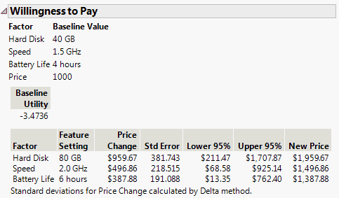
The Willingness to Pay report displays the baseline value for each factor, as well as baseline utility values. For each factor, the report shows the feature setting, estimated price change, and new price. If there are no interaction or second-order effects, standard errors and confidence intervals are also shown. These are calculated using the delta method.
Figure 4.21 Willingness to Pay Report
 Save Bayes Chain
(Available for models fit with Hierarchal Bayes.) You can use the Bayes Chain data table to determine whether your estimates have stabilized. The table that is created has a number of rows equal to the Number of Bayesian Iterations (specified on the launch window) plus one. The first row, Iteration 1, gives the starting values. Subsequent rows show the results of the iterations, in order. The table has a column for the iteration counts, the model Log Likelihood, and columns corresponding to each model effect:
Iteration
Gives the iteration number, where the first row shows starting values.
Log Likelihood
The log-likelihood of the model for that iteration. You can plot the Log Likelihood against Iteration to view behavior over the burn-in and tuning periods.
Adaptive Sigma for <model effect>
Gives the estimate of the square root of the diagonal entries of the inverse Wishart distribution scale matrix for the corresponding effect.
Acceptance for <model effect>
Gives the sampling acceptance rate for the corresponding effect.
Mean of <model effect>
Gives the estimated mean for the corresponding effect.
Variance of <model effect>
Gives the estimated variance for the corresponding effect.

