Interpret the Profiles
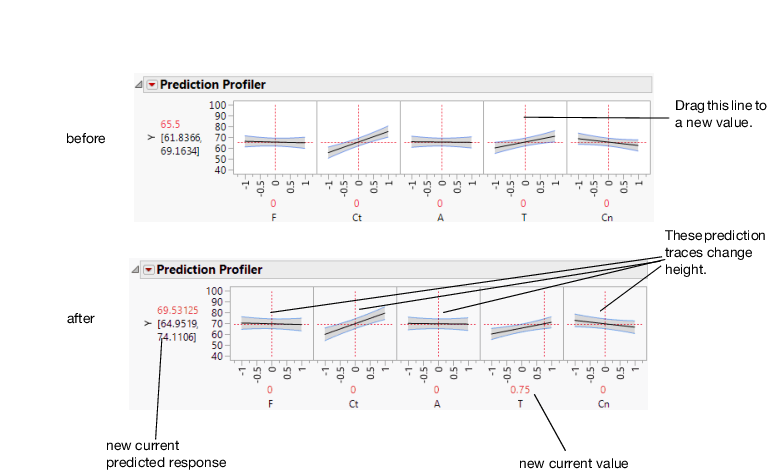
The illustration in Figure 2.4 describes how to use the components of the Prediction Profiler. There are several important points to note when interpreting a prediction profile:
• The importance of a factor can be assessed to some extent by the steepness of the prediction trace. If the model has curvature terms (such as squared terms), then the traces might be curved.
• If you change the value of a factor, the prediction trace for that factor is not affected, but the prediction traces of all the other factors can change. The Y response line must cross the intersection points of the prediction traces with their current value lines.
Note: If there are interaction effects or cross-product effects in the model, the prediction traces can shift their slope and curvature as you change current values of other terms. That is what interaction is all about. If there are no interaction effects, the traces change only in height, not slope or shape.
Figure 2.4 Changing One Factor from 0 to 0.75
Prediction profiles are especially useful in multiple-response models to help judge which factor values can optimize a complex set of criteria.
Click a graph or drag the current value line right or left to change the factor’s current value. The response values change as shown by a horizontal reference line in the body of the graph. Double-click in an axis to bring up a window that changes its settings.
The Profiler as a Cross-Section
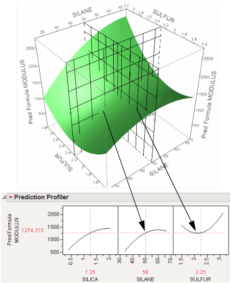
In the following example using Tiretread.jmp, look at the response surface of the expression for MODULUS as a function of SULFUR and SILANE (holding SILICA constant). Now look at how a grid that cuts across SILANE at the SULFUR value of 2.25. Note how the slice intersects the surface. If you transfer that down below, it becomes the profile for SILANE. Similarly, note the grid across SULFUR at the SILANE value of 50. The intersection when transferred down to the SULFUR graph becomes the profile for SULFUR.
Figure 2.5 Profiler as a Cross-Section
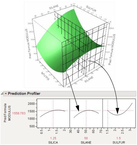
Now consider changing the current value of SULFUR from 2.25 to 1.5.
Figure 2.6 Profiler as a Cross-Section
In the Prediction Profiler, note the new value just moves along the same curve for SULFUR, the SULFUR curve itself does not change. But the profile for SILANE is now taken at a different cut for SULFUR. The profile for SILANE is also a little higher and reaches its peak in the different place, closer to the current SILANE value of 50.
Set or Lock Factor Values
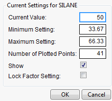
If you press Alt (Option on macOS) and click in a graph, a window prompts you to enter specific settings for the factor.
Figure 2.7 Continuous Factor Settings Window
For continuous variables, you can specify the following:
Current Value
The value used to calculate displayed values in the profiler, equivalent to the red vertical line in the graph.
Minimum Setting
The minimum value of the factor’s axis.
Maximum Value
The maximum value of the factor’s axis.
Number of Plotted Points
Specifies the number of points used in plotting the factor’s prediction traces.
Show
Show or hide the factor in the profiler.
Lock Factor Setting
Locks the value of the factor at its current setting.


