Response Surface Design with Flexible Blocking
When optimizing a process, you might need to include qualitative factors in your experiment as well as continuous factors. You might need to block by qualitative factors such as batch or day, or include qualitative factors such as machine or delivery mechanism. But the Response Surface Design platform supports only continuous factors. To obtain a response surface design with a qualitative factor, you can replicate the design over each level of the factor. However, this is inefficient. The Custom Design platform constructs an optimal design with fewer runs.
In this example, you construct a response surface design that accommodates two continuous factors and a blocking factor with four runs per block. You can include categorical or discrete numeric factors in a similar fashion.
1. Select DOE > Custom Design.
2. Type 2 next to Add N Factors.
3. Click Add Factor > Continuous.
4. Click Add Factor > Blocking > 4 runs per block.
Notice that only one level appears under Values. This is because the number of blocks cannot be determined until the number of runs is determined.
Figure 5.35 Factors Outline with Two Continuous Factors and a Blocking Factor
5. Click Continue.
The Default number of runs is 12. The Factors outline updates to show three levels for the Blocking factor, X3. Because you required X3 to have four runs per block, the 12 runs allow three blocks.
6. Click RSM.
An informational JMP Alert window reminds you that the blocking factor cannot appear in interaction or quadratic terms. JMP adds only the appropriate RSM terms to the list.
7. Click OK to dismiss the message.
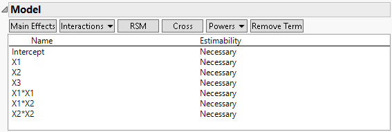
Quadratic and interactions terms for X1 and X2 are added to the model. Because you added RSM terms, the Recommended optimality criterion changes from D-Optimal to I-Optimal. You can see this later in the Design Diagnostics outline.
Figure 5.36 Model Outline with Response Surface Effects
Note: Setting the Random Seed in step 8 and Number of Starts in step 9 reproduces the exact results shown in this example. In constructing a design on your own, these steps are not necessary.
8. (Optional) Click the Custom Design red triangle, select Set Random Seed, type 12345, and click OK.
9. (Optional) Click the Custom Design red triangle, select Number of Starts, type 5, and click OK.
10. Click Make Design.
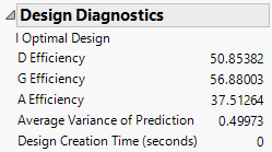
11. Open the Design Evaluation > Design Diagnostics outline.
Figure 5.37 Design Diagnostics Outline
The first line in the Design Diagnostics outline identifies the optimality criterion being used. This design is I-optimal.
12. Click Make Table.
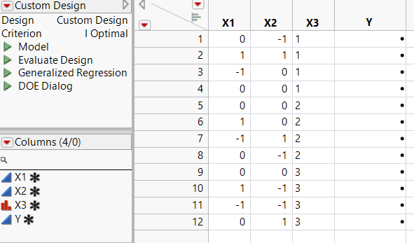
Figure 5.38 Design Table with Blocking Factor
Because the default Run Order was Randomize within Blocks, the levels of the blocking factor (X3) are sorted.
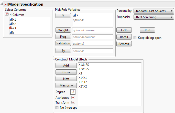
13. In the Table panel of the design table, click the green triangle next to the Model script.
Figure 5.39 Fit Model Window
Notice the following:
– The blocking factor (X3) is entered as an effect.
– No interactions involving X3 are included.
– The other five effects define a response surface model for X1 and X2.


