Example of a Probit Model with Binomial Errors: Numerical Derivatives
The Ingots2.jmp sample data table includes the numbers of ingots tested for readiness after different treatments of heating and soaking times. The response variable, NReady, is binomial, depending on the number of ingots tested (Ntotal) and the heating and soaking times. Maximum likelihood estimates for parameters from a probit model with binomial errors are obtained using:
• numerical derivatives
• the negative log-likelihood as a loss function
• the Newton-Raphson method.
The average number of ingots ready is the product of the number tested and the probability that an ingot is ready for use given the amount of time it was heated and soaked. Using a probit model, the P column contains the model formula:
Normal Distribution(b0+b1*Heat+b2*Soak)
The argument to the Normal Distribution function is a linear model of the treatments.
To specify binomial errors, the loss function, Loss, has the formula
-(Nready*Log(p) + (Ntotal - Nready)*Log(1 - p))
Follow these steps to fit the model:
1. Select Help > Sample Data Library and open Ingots2.jmp.
2. Select Analyze > Specialized Modeling > Nonlinear.
3. Assign P to the X, Predictor Formula role,
4. Assign Loss to the Loss role.
5. Select the Numeric Derivatives Only option.
6. Click OK.
7. Click Go.
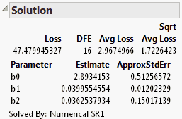
The platform used the Numerical SR1 method to obtain the parameter estimates shown in Figure 15.15.
Figure 15.15 Solution for the Ingots2 Data
