Properties That Control How Columns Are Used in Platforms
The following properties control how columns are used in platforms:
• Distribution
• Time Frequency
• Map Role
• Supercategories
• Multiple Response
• Target Level
• Profit Matrix
• Informative Missing
Distribution
For a column that contains continuous numeric data, use the Distribution property to select a distribution type to fit to the column. This distribution is used in the Distribution platform and is used in the Process Capability platform under certain conditions. See Distribution and Process Capability Distribution.
When you obtain a Distribution report (by selecting Analyze > Distribution) for the column, JMP automatically estimates a fit using the specified distribution. A curve representing the fitted distribution is superimposed on the histogram.
If you set both the Distribution property and the Spec Limits property, then the Distribution platform produces a Capability Analysis report that is based on the distribution specified in the Distribution column property.
Note: In older data tables, the Capability Analysis column property might have been assigned to a column to specify spec limits. We recommend that you use the Spec Limits property instead.
Distribution and Process Capability Distribution
If you are using the Process Capability platform to analyze a column that does not contain a Process Capability Distribution property, the distribution specified in the Distribution column property results in a nonnormal fit in the Process Capability platform. If this distribution is supported in the Process Capability platform, then it is used. However, if this distribution is not supported, the platform uses a Johnson fit.
If both the Distribution and Process Capability Distribution column properties are saved for a given column, then the distribution specified in the Distribution column property is used in the Distribution platform, and the distribution specified in the Process Capability Distribution column property is used in the Process Capability platform.
Time Frequency
When using the Time Series platform, you can assign the Time Frequency property to data. The Time Frequency property specifies the frequency with which the data is reported (such as annually, quarterly, monthly, and so on). Specifying a time frequency allows JMP to take things like leap years and leap days into account. If no frequency is specified, the data is treated as equally spaced numeric data.
Map Role
If you have created a data table that contains boundary data (such as countries, states, provinces, or counties), to see a corresponding map in Graph Builder, use the Map Role property.
Note the following:
• If the custom boundary files reside in the default custom maps directory, then you need to specify only the Map Role property in the -Name file.
• If the custom boundary files reside in an alternate location, then you must specify the Map Role property in the -Name file and in the data table that you are analyzing.
• The columns that contain the Map Role property must contain the same boundary names, but the column names can be different.
For an example using the Map Role property, see Map Role in Essential Graphing.
To add the Map Role property into the -Name data table
1. Right-click the column containing the boundaries and select Column Properties > Map Role.
2. Select Shape Name Definition.
3. Click OK.
4. Save the data table.
To add the Map Role property into the data table that you are analyzing
Note: Perform these steps only if your custom boundary files do not reside in the default custom maps directory.
1. Right-click the column containing the boundaries and select Column Properties > Map Role.
2. Select Shape Name Use.
3. Next to Map name data table, click ![]() to browse to a -Name map data table. You can enter the relative or absolute path.
to browse to a -Name map data table. You can enter the relative or absolute path.
If the map data table is in the same folder, enter only the filename. Quotation marks are not required when the path contains spaces.
4. Next to Shape definition column, enter the name of the column in the map data table whose values match those in the selected column.
5. Click OK.
6. Save the data table.
When you generate a graph in Graph Builder and assign the modified column to the Shape zone, your boundaries appear on the graph.
Supercategories
When a data set contains ratings (for example, on a five-point scale), you might want to know the percent of the responses in a subset of those ratings. Add a Supercategories column property to group specific categories into one category.
Supercategories are supported only in the Categorical platform.
To add the Supercategory property to a data column
1. Right-click the column that contains categories that you want to group.
2. Select Column Properties > Supercategories.
The column properties window shows the Supercategories options (Figure 5.5).
3. Select the categories in the Column’s Categories list that you want to group.
4. Enter a descriptive name next to Supercategory Name.
Leave the name blank, and JMP names the supercategory after the categories that you selected.
5. Click Add to create the supercategory.
6. Click the Supercategories red triangle and select from the following options:
Options > Hide
Hides data in the selected supercategory from reports and graphs.
Add All
Creates a supercategory from all of the categories in the column.
Add Mean and Add Std Dev
Calculate statistics for value scores. See Consumer Research.
7. Click OK to add the property to the column.
Figure 5.5 Example of a Supercategories Configuration
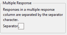
Multiple Response
The term multiple response refers to the situation where the cells in a column contain more than one response value. For example, many cells in the Brush Delimited column in the Consumer Preferences.jmp sample data table contain multiple values. For example, row 6 contains “Wake, After Meal, Before Sleep”.
Add the Multiple Response column property if you want to specify a delimiter other than the comma. Otherwise, change the column’s modeling type to Multiple Response in the Column Info window. See About Modeling Types for more information about the Multiple Response modeling type.
JMP automatically assigns the Multiple Response modeling type to data tables saved in JMP 12 or lower. The column must contain the Multiple Response column property, and the delimiter must be a comma for the automatic assignment to take place. JMP does not remove the Multiple Response column property, though you might choose to do so.
Figure 5.6 Multiple Response Configuration Window
Note: You can use the Multiple Response property in the Categorical platform. See Multiple Response in Consumer Research. You can also use this property in the Data Filter. See The Data Filter. If the delimiter is a comma, consider using the Multiple Response modeling type instead.
Target Level
Use the Target Level column property to specify the level of interest of a response column for logistic regression platforms. This level is used as the positive response level in logistic regression models, and it impacts the statistics, probability curves, and other measures of fit. This column property is designed for binary responses, but it can be used for any categorical column.
Note: The Target Level column property is used by the following platforms when a binary response column is specified: Fit Y by X (Logistic) and the Nominal Logistic personality of Fit Model.
Profit Matrix
Use the Profit Matrix column property to assign weights to the levels of a nominal or ordinal response variable for a predictive model. For a nominal response, you can specify the profit matrix entries using a probability threshold.
Note: The Profit Matrix column property is used by the following platforms: Model Comparison, Partition, PLS, and Fit Model. The personalities in Fit Model that use the Profit Matrix column property are Generalized Regression, Nominal Logistic, and Ordinal Logistic.
Profit Matrix
When you select Column Properties > Profit Matrix, a matrix template appears, with a row and column for each value in the selected column. The Actual levels are shown as rows and the predicted levels are shown as columns. Correct decisions are those on the diagonal, where the predicted level equals the actual level.
• For diagonal entries, enter values that reflect profits or weights for correct decisions.
• For non-diagonal entries, enter values that reflect profits (or losses) or weights for incorrect decisions.
• For situations where no prediction is made, use the Undecided column to indicate associated profits or losses.
Probability Threshold Specification for Profit Matrix
When the response is binary, additional options appear beneath the profit matrix template. These options enable you to specify a probability threshold instead of entering weights directly into the profit matrix.
Specify the Target Level and Probability Threshold. Then click Set to update the profit matrix.
Target Level
The level whose probability is modeled.
Probability Threshold
A threshold for the probability of the target level. If the probability that an observation falls into the target level exceeds the probability threshold, the observation is classified into that level.
Set
Enters values into the profit matrix template that reflect your specifications for Target and Probability Threshold. See Probability Threshold Calculations.
Probability Threshold Calculations
Denote the threshold probability by t. When you click Set, the entries in the profit matrix are assigned as follows:
• 0 for each diagonal entry, reflecting no loss from correct decisions
• -1 for a prediction of the target level when the actual value is the non-target level
• -t/(1 - t) for a prediction of the non-target level when the actual value is the target level
This implies that the profits for classifying into the two levels are given as follows:


The Most Profitable Prediction is the level whose profit is the larger of these two values. It follows from the two Profit equations above that an observation is assigned to the target level whenever Prob[Target Level] is at least t.
Profit Matrix and Predictive Models
For a nominal or ordinal column with the Profit Matrix column property, most modeling platforms enable you to save formula columns that reflect profit matrix entries. Fit your model and then select the Save Prediction Formula or Save Probability Formula option. In addition to saving the usual prediction formulas to the data table, JMP saves the following analogs of the usual formula columns:
• Profit for <level>: For each level of the response, a column gives the expected profit for classifying each observation into that level.
• Most Profitable Prediction for <column name>: For each observation, gives the level of the response with the highest expected profit.
• Expected Profit for <column name>: For each observation, gives the expected profit for the classification defined by the Most Profitable Prediction column.
• Actual Profit for <column name>: For each observation, gives the actual profit for classifying that observation into the level specified by the Most Profitable Prediction column.
See Example of a Profit Matrix for More Than Two Levels. For an example of using a profit matrix in modeling, see Decision Matrix Report in Predictive and Specialized Modeling.
Example of a Profit Matrix for More Than Two Levels
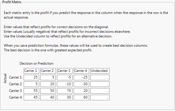
The example below shows a profit matrix for the Airline column in the Travel Costs.jmp sample data table.
Figure 5.7 Example of Profit Matrix Window
To see how the values in this profit matrix were assigned, consider a travel agency that uses four airlines, Carrier 1 to Carrier 4, to service its customers. For each ticket sold, the agency realizes a profit that depends on the carrier selected by the customer. When the agency recommends, or predicts, a carrier, it reserves a ticket for a small fee. If the customer decides to use the predicted carrier, the agency profits by a certain amount less the reservation fee. However, if the customer decides to take a different carrier, the agency loses the reservation fee and must pay another reservation fee. The agency’s profit is lower due to the incorrect prediction.
Suppose that the reservation fees for Carriers 1 through Carrier 4 are $15, $20, $30, and $50, respectively, and that the profits from ticket sales are $40, $40, $100, and $110, respectively.
If the agency recommends Carrier 1 to a customer who then decides to purchase the ticket, the agency reserves a ticket for $15 and then receives $40 for a net profit of $25. If the agency predicts that a customer will choose Carrier 4 but the customer chooses Carrier 1, the agency loses $50 for the Carrier 4 reservation and must also pay $15 for the reservation on Carrier 1. This gives the agency a net loss of $40 - $50 - $15 = -$25.
Example of Using Probability Threshold to Define the Profit Matrix
The sample data table Liver Cancer.jmp gives disease Severity ratings for 136 patients. You are interested in modeling Severity using the predictors given in the columns from BMI to Jaundice. The usual prediction formulas for a model classify a patient into the Severity level that is most probable. However, classifying a patient as having Low severity when in actuality the patient’s severity is High is a more costly error than classifying a patient as having High severity when in actuality the patient’s severity is Low. As a result, you want to assign a higher cost to misclassifying a patient as Low, when the patient’s severity is actually high.
You can assign this higher cost by setting a probability threshold. With input from experts, you determine that the following is a good strategy: Classify into the High level of Severity any patient whose predicted probability of being in the High level exceeds 0.4.
1. Select Help > Sample Data Library and open Liver Cancer.jmp.
2. Select the Severity column and select Cols > Column Info.
3. Select the Profit Matrix column property.
4. Change the Target to High.
5. Enter 0.4 as the Probability Threshold.
6. Click Set.
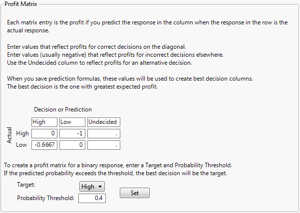
The profit matrix updates to show the corresponding weights.
Figure 5.8 Profit Matrix Showing Weights Corresponding to Probability Threshold
The profit matrix shows that the loss for misclassifying a patient with High severity as having Low severity is -1, while the loss for misclassifying a patient with Low severity as having High severity is smaller, -0.6667.
Informative Missing
The Informative Missing column property directs most fitting platforms to use a coding system for columns that contain missing values. For continuous columns, the coding system consists of two columns. The first column is a column of the original values with missing values replaced by the mean of the nonmissing values; the second column is an indicator column to denote which rows are missing. For categorical columns, missing values are treated as a distinct level of the column.


