Example of a Transfer Function Model
Use the Time Series Analysis platform to find a transfer function to model the input and output of a gas furnace. Identifying an appropriate transfer function is an iterative process. In this example, the input function is the methane gas feed rate measured in cubic feet per minute and the output function is the percent carbon dioxide in the gas that is produced. For a full treatment of the example, see Box et al. (1994).
Launch the Time Series Analysis Platform
1. Select Help > Sample Data Folder and open Time Series/seriesJ.jmp.
2. Select Analyze > Specialized Modeling > Time Series.
3. Select Output CO2 and click Y, Time Series.
4. Select Input Gas Rate and click Input List.
5. Click OK.
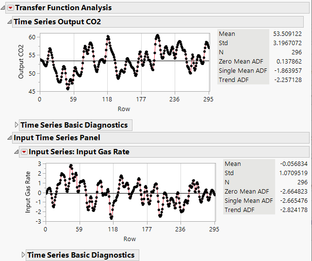
Figure 18.27 Initial Transfer Function Report
Since an input variable was specified in the launch window, a Transfer Function Analysis report is shown instead of a Time Series Analysis report. The initial report contains a section for the output series and a section for the input series. Each section provides a graphical representation of the series and basic diagnostics.
6. In the Input Time Series Panel section, click the triangle next to Time Series Basic Diagnostics.
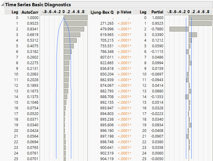
Figure 18.28 Diagnostics for Input Gas Rate
The Time Series Basic Diagnostics report shows autocorrelations and partial autocorrelations for the input series. There are no cyclical patterns in the correlations that would indicate a significant seasonal trend in the data. Therefore, you do not need to consider seasonal parameters when specifying your transfer model.
Prewhitening the Input Data
The prewhitening technique is used to help identify the transfer function model. The goal is to find an ARIMA model that provides a good fit for the input series. You can use the input diagnostics to determine which type of ARIMA model to fit to Input Gas Rate. In the partial autocorrelation plot, which is found in the Time Series Basic Diagnostics section, there is a sharp cutoff of significant correlations with the last significant partial autocorrelation at Lag 3. This indicates that an AR(3) model might be an appropriate ARIMA model for the input series. You can check this by fitting an AR(3) model separately, prior to using it in the prewhitening step.
1. Click the red triangle next to Input Series: Input Gas Rate and select ARIMA.
2. In the ARIMA Specification window, type 3 next to p, Autoregressive Order.
3. Click Estimate.
4. Scroll down to the Residuals and click the triangle next to Residuals to view.
The residuals are small and do not have a distinct pattern. The autocorrelations and partial autocorrelations are also not significant. These observations confirm that AR(3) is an appropriate ARIMA model to use in the prewhitening step.
5. Click the red triangle next to Input Series: Input Gas Rate and select Prewhitening.
6. In the Non-Seasonal Order section of the Prewhitening Specification window, type 3 next to p, Autoregressive Order.
7. Click Estimate.
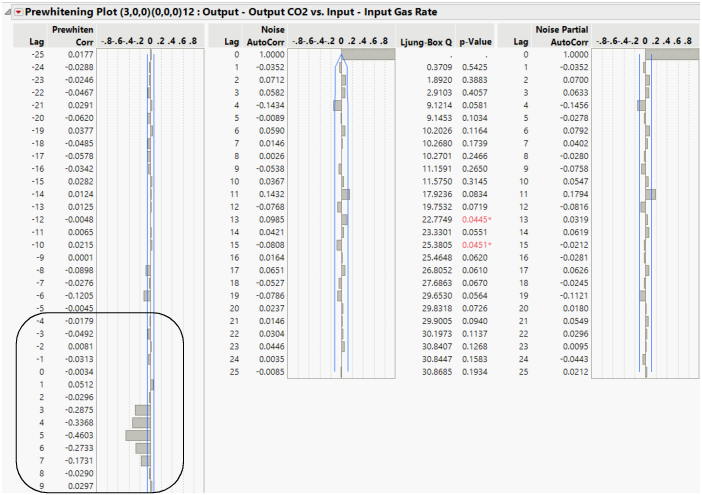
Figure 18.29 Prewhitening Report
Use the prewhitening results to help identify the transfer function. The outlined portion in Figure 18.29 is the graphical representation of the transfer function. For those less familiar with transfer functions, there is a table in Box et al. (1994) that illustrates what transfer functions look like based on different specifications. According to this table, the pattern of the transfer function corresponds to orders 1 or 2 for both the numerator, ω(B), and denominator, δ(B). See Statistical Details for Transfer Functions for the mathematical specifications of the transfer function. For this example, m = 1, which indicates that there is only one pair of ω(B) and δ(B).
In addition, the first significant nonzero cross-correlation is at Lag 3. The next steps of this example assume an order of 2 for both the numerator and denominator of the transfer function and 3 for the lag, and then fit a preliminary transfer function model.
Fit a Preliminary Transfer Function Model
1. Click the Transfer Function Analysis red triangle and select Transfer Function.
2. In the Transfer Function Model Specification window, set the following specifications:
– Type 2 next to s1, Order of Numerator Operator.
– Type 2 next to r1, Order of the Denominator Operator.
– Type 3 next to L, Input Lag.
– Type 12 next to Forecast Periods.
3. Click Estimate.
4. Click the triangle next to the Residuals section of the Transfer Function Model (1) report.
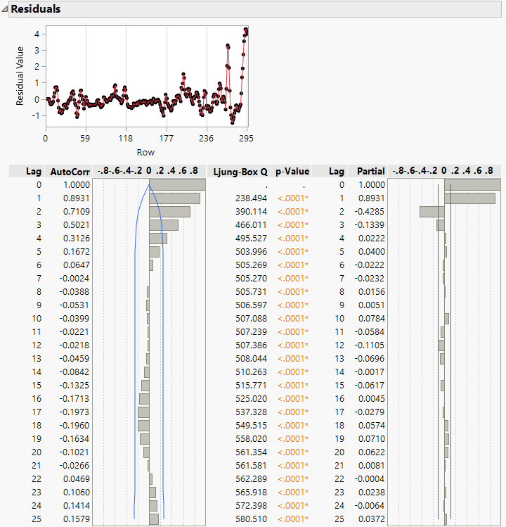
Figure 18.30 Residuals for the Preliminary Transfer Function Model
The residuals plot shows that the residuals increase towards the end of the series. Also, there are significant autocorrelations and partial autocorrelations. This indicates that the preliminary transfer function model has not addressed the autocorrelation among the residuals. To better fit the data, the noise series needs to be modeled appropriately. We can look at the partial autocorrelations and see that there is a cutoff of significant correlations at Lag 2. This indicates that perhaps an AR(2) model is appropriate for the noise series.
5. Click the Transfer Function Analysis red triangle and select Transfer Function.
6. In the Transfer Function Model Specification window, set the following specifications:
– Type 2 next to p, Autoregressive Order.
– Type 2 next to s1, Order of Numerator Operator.
– Type 2 next to r1, Order of the Denominator Operator.
– Type 3 next to L, Input Lag.
– Type 12 next to Forecast Periods.
7. Click Estimate.
Figure 18.31 Transfer Function Analysis Model Comparison Report
The Model Comparison report indicates that the second transfer function model is a better fit. The second model has a lower AIC and a higher RSquare than the first model.
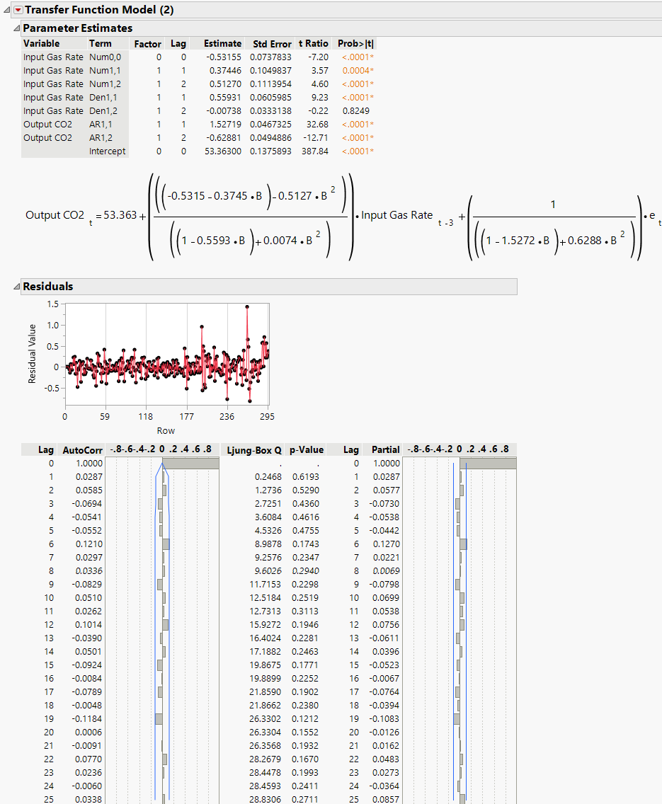
8. Scroll to the report for Transfer Function Model (2).
Figure 18.32 Final Transfer Function Model Report
There is no longer autocorrelation among the residuals, which indicates that this transfer function model is an appropriate model. The model equation is displayed in the report.
