Elements Common to Most Personalities 

Model Specification	The red triangle menu next to Model Specification contains options that enable you to: • Center effects when polynomials are included in the model • Codes for missing values • Set the alpha level for confidence intervals • Save the model specifications to a script window or to a script attached to the data table • Interact with SAS • Set convergence criteria See Model Specification Options.
Select Columns	Lists the unexcluded columns in the current data table.
Y	Identifies one or more response variables (the dependent variables) for the model.
Weight	Identifies a column whose values assign a weight to each row for the analysis. See Weight.
Freq	Identifies a column whose values assign a frequency to each row for the analysis. In general terms, the effect of a frequency column is to expand the data table, so that any row with integer frequency k is expanded to k rows. You are allowed to specify fractional frequencies. See Frequency.
Validation	In JMP Pro, for some personalities, you can enter a Validation column. See the appropriate Personality chapter for details. If you click the Validation button with no columns selected in the Select Columns list, you can add a validation column to your data table. For more information about the Make Validation Column utility, see Basic Analysis.
By	Performs a separate analysis for each level of the variable.
Add	Adds effects to the model. See Add.
Cross	Creates interaction and polynomial effects by crossing two or more variables. See Cross.
Nest	Creates nested effects. See Nest.
Macros	Automatically generates effects for commonly used models. See Macros.
Degree	Applies the specified degree to models with factorial or polynomial effects generated using Macros. See Factorial to Degree and Polynomial to Degree in Macros.
Attributes	Applies attributes to model effects. These attributes determine how the effects are treated. See Attributes.
Transform	Transforms selected continuous effects or Y columns. See Transform.
No Intercept	Excludes the intercept term from the model.
Personality	Specifies the fitting methodology. See Fit Model Launch Window Elements. Different options appear depending on the personality that you select.
Help	Takes you to Help topics for the Fit Model launch window.
Recall	Populates the launch window with the last model specification that you ran.
Remove	Removes the selected variable from the assigned role. Alternatively, double click the effect or select the effect and press the Backspace key.
Run	Generates the report window for the specified model and personality.
Keep dialog open	Keeps the launch window open after you run the analysis, enabling you to alter and re-run the analysis at any time.

Descriptions of the Macros Options 

Full Factorial	Creates all main effects and interactions for the columns selected in the Select Columns list. These are entered in an order that is based on the order in which the main effects are listed in the Select Columns list. For an alternate ordering, see Factorial Sorted, in this table.
Factorial to Degree	Creates all main effects, but only interactions up to a specified degree (order). Specify the degree in the Degree box beneath the Macros button.
Factorial Sorted	Creates the same set of effects as the Full Factorial option but lists them in order of degree. All main effects are listed first, followed by all two-way interactions, then all three-way interactions, and so on.
Response Surface	Creates main effects, two-way interactions, and quadratic terms. The selected main effects are given the response surface attribute, denoted RS. When the RS attribute is applied to main effects and the Standard Least Squares personality is selected, a Response Surface report is provided. This report gives information about critical values and the shape of the response surface. See also Response Surface Effect in Attributes and the Design of Experiments Guide.
Mixture Response Surface	Creates main effects and two-way interactions. Main effects have the response surface (RS) and mixture (Mixture) attributes. In the Standard Least Squares personality, the Mixture attribute causes a mixture model to be fit. The RS attribute creates a Response Surface report that is specific to mixture models. See also Mixture Effect in Attributes and the Design of Experiments Guide.
Polynomial to Degree	Creates main effects and polynomial terms up to a specified degree. Specify the degree in the Degree box beneath the Macros button.
Scheffé Cubic	Creates main effects, interactions, and Scheffé cubic terms, which are useful in specifying response surfaces for mixture experiments. This macro creates a complete cubic model. When you fit a 3rd degree polynomial model to a mixture, you must not introduce even-powered terms, for example X1*X1*X2, because they are not estimable. However, it turns out that a complete polynomial specification of the surface can include terms of the form X1*X2*(X1 – X2), which are called Scheffé cubic terms. Scheffé cubic terms are also included if you enter a 3 in the Degree box and then select the Mixture Response Surface macro command.
Radial	Fits a radial smoother using the selected variables. The number of knots is the number of unique values of the smoothing variable. The smoother is based on the automatic smoother in Ruppert, Wand, and Carroll (2003, Chapter 13.4–13.5). This produces the same results as does the GLIMMIX procedure in SAS/STAT if the following options are included in the RANDOM statement: TYPE=RSMOOTH, KNOTMETHOD=DATA.

Descriptions of the Attributes Options 

Random Effect	Assigns the Random attribute to an effect. For details about random effects, see Specifying Random Effects and Fitting Method in Standard Least Squares Report and Options.
Response Surface Effect	Assigns the RS attribute to an effect. Note that the relevant model terms must be included in the Construct Model Effects list. The Response Surface option in the Macros list automatically generates these terms and assigns the RS attribute to the main effects. To obtain the Response Surface report, interaction and polynomial terms do not need to have the RS attribute assigned to them. You need only assign this attribute to main effects.
LogVariance Effect	Assigns the LogVariance attribute to an effect. This attribute indicates that the effect is to be included in a model of the variance of the response. To include an effect in models for both the mean and variance of the response, you must specify the effect twice. In the tabbed interface, it must appear on both the Mean Effects and Variance Effects tabs. Otherwise, you can enter it twice on the Mean Effects tab, once without the LogVariance Effect attribute and once with the LogVariance Effect attribute.
Mixture Effect	Assigns the Mixture attribute to main effects. This is used to specify the main effects involved in the mixture. Note that the Mixture Response Surface option in the Macros list automatically assigns the mixture attribute to selected effects, and provides a Response Surface report when possible.
Excluded Effect	Assigns the Excluded attribute to an effect. This excludes the effect from the model fit. However, the effect is used to group observations for lack-of-fit tests. In the Standard Least Squares personality, a table of least square means is provided for this effect.
Knotted Spline Effect	Assigns the Knotted attribute to a continuous main effect. This implicitly adds cubic splines for the effect to the model specification. See Knotted Spline Effect.

Descriptions of the Transform Options 

None	Removes any Transform options that have been applied.
Log	Applies the natural logarithm transformation to the selected variable.
Sqrt	Takes the square root of the values of the selected variable.
Square	Squares the values of the selected variable.
Reciprocal	Applies the transformation 1/X to the variable X.
Exp	Applies the exponential transformation to the selected variable.
Arrhenius	Applies the Arrhenius transformation to the variable T (temperature in degrees Centigrade): This is the component of the Arrhenius relationship that is multiplied by the activation energy.
ArrheniusInv	Applies the inverse of the Arrhenius transformation to the variable X:
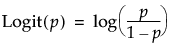
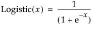
Logit	Calculates the inverse of the logistic function for the selected column (where p is in the range of 0 to 1):
Logistic	Calculates the logistic (also known as Squish and Logist) function for the selected column (where the result is in the range of 0 to 1):
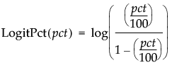
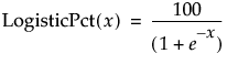
LogitPct	Calculates the logit as a percent for the selected column (where pct is a percent in the range of 0 to 100):
LogisticPct	Calculates the logistic (or logist) as a percent for the selected column (where the result is in the range of 0 to 100):

Description of Personalities with Tabbed Construct Model Effects Input 

Standard Least Squares	Fixed Effects tab: Enter effects to be modeled as fixed effects. A fixed effect is one whose specific treatment levels are of interest. You want to compare the mean response across its treatment levels. Random Effects tab: Enter effects to be modeled as random effects. A random effect is one whose levels are considered a random sample from a larger population. You want to estimate the variation in the response that is attributable to this effect.
Mixed Model	Fixed Effects tab: Enter effects to be modeled as fixed effects. See Standard Least Squares in this table. Random Effects tab: Enter effects to be modeled as random effects. Use for variance component models and random coefficients models. Repeated Structure tab: Use to select a covariance structure for repeated effects.
LogLinear Variance	Mean Effects tab: Enter effects for which you want to model expected values. Variance Effects tab: Enter effects for which you want to model variance. If you want to model both the expected value and variance of an effect, you must enter it on both tabs.
Parametric Survival	Location Effects tab: Enter effects that you want to use in modeling the location parameter, mu, or in the case of the Weibull distribution, the shape parameter. Scale Effects tab: Enter effects that you want to use in modeling the scale parameter.

Description of Fitting Personalities 

Personality	Description	Reference
Standard Least Squares	Fits models where the response is continuous. Techniques include regression, analysis of variance, analysis of covariance, mixed models, and analysis of designed experiments.	Standard Least Squares Report and Options section Emphasis Options for Standard Least Squares
Stepwise	Facilitates variable selection for standard least squares and ordinal logistic analyses (or nominal with a binary response). For continuous responses, cross validation, p-value, BIC, and AICc criteria are provided. Also provided are options for fitting all possible models and for model averaging. For logistic fits, p-value, BIC, and AICc criteria are provided.	Stepwise Regression Models section
Generalized Regression	Fits generalized linear models using regularized, also known as penalized, regression techniques. The regularization techniques include ridge regression, the lasso, the adaptive lasso, the elastic net, and the adaptive elastic net. The response distributions include the normal, binomial, Poisson, zero-inflated Poisson, negative binomial, zero-inflated negative binomial, and gamma.	Generalized Regression Models section Distribution
Mixed Model	Fits a wide variety of linear models for continuous-responses with complex covariance structures. The situations addressed include: ‒ Split plot experiments ‒ Random coefficients models ‒ Repeated measures designs ‒ Spatial data ‒ Correlated response data	Mixed Models section
Manova	Fits models that involve multiple continuous Y variables. Techniques include multivariate analysis of variance, repeated measures, discriminant analysis, and canonical correlations.	Multivariate Response Models section
LogLinear Variance	For a continuous Y variable, constructs models for both the mean and the variance. You can specify different sets of effects for the two models.	Loglinear Variance Models section
Nominal Logistic	Fits a logistic regression model to a nominal response.	Logistic Regression with Nominal or Ordinal Responses section
Ordinal Logistic	Fits a logistic regression model to an ordinal response.	Logistic Regression with Nominal or Ordinal Responses section
Proportional Hazard	Fits a semi-parametric regression model (the Cox proportional hazards model) to assess the effect of explanatory variables on survival times, taking censoring into account. You can also launch this personality by selecting Analyze > Reliability and Survival > Fit Proportional Hazards.	See the Reliability and Survival Methods book.
Parametric Survival	Fits a general linear regression model to survival times. Use this option if you have survival times that can be expressed as a function of one or more explanatory variables. Takes into account various survival distributions and censoring. You can also launch this personality by selecting Analyze > Reliability and Survival > Fit Parametric Survival.	See the Reliability and Survival Methods book.
Generalized Linear Model	Fits generalized linear models using various distribution and link functions. Techniques include logistic, Poisson, and exponential regression.	Generalized Linear Models section
Partial Least Squares	Fits models to one or more Ys using latent factors. This permits models to be fit when explanatory variables (Xs) are highly correlated, or when there are more Xs than observations. You can also launch a partial least squares analysis by selecting Analyze > Multivariate Methods > Partial Least Squares.	See the Multivariate Methods book.
Response Screening	Automates the process of conducting tests for linear model effects across a large number of responses. Test results and summary statistics are presented in data tables and plots. A False-Discovery Rate (FDR) approach guards against incorrect declarations of significance. A robust estimation method reduces the sensitivity of tests to outliers. Note: This personality only allows continuous responses. Response Screening for individual factors is also available by selecting Analyze > Modeling > Response Screening. This platform supports categorical responses, and also provides equivalence tests and tests of practical significance.	See the Specialized Models book.