Findings Distribution
This report compares distributions of Findings and demographic variables across treatment arms.
Note: JMP Clinical uses a special protocol for data including non-unique Findings test names. Refer to How does JMP Clinical handle non-unique Findings test names? for more information.
Note: Refer to Distribution Reports for a description of the general analysis performed by the JMP Clinical distribution reports.
Note: If FAOBJ is found, JMP Clinical will draw distributions for the object of observation and will run both contingency and oneway analyses for each test group by the object of observation.
Report Results Description
Running Findings Distribution for Nicardipine using default settings generates the Report shown below.
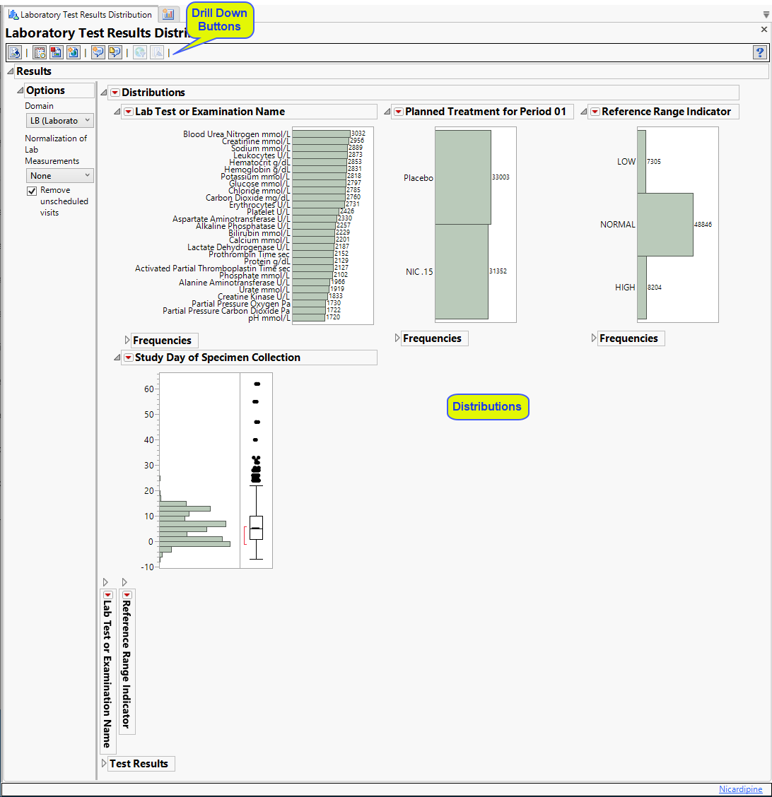
The Report contains the following sections:
Distributions
Contains Histograms to display the distribution of Findings tests taken during the study and other relevant variables for the selected Findings domain.
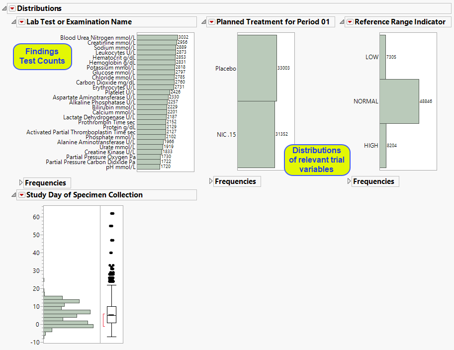
| • | One Findings Test Counts Graph. |
This graph shows a Histogram displaying how often measurements were taken for each findings test (xxTESTCD) during the study.
| • | A set of Distributions. |
These display counts and histograms of relevant variables in the Findings data set. A distribution of subjects on the Actual, Planned, or Specified Treatment is shown as well as other findings variables (if present). Findings variables displayed can include the Findings Body System (xxBODSYS), Reference Range Indicator1 (xxNRIND), the Category for the Test (xxCAT) and Subcategory (xxSCAT), the Categorical Findings Result (xxSTRESC, only displayed for categorical findings domains), the Visit and Time Points at which findings were taken (VISIT and xxTPT), Baseline Flag (xxBLFL), and the Study Day.
These distributions are useful for understanding the frequency and details of findings tests taken during a study. All distributions are linked: You can select bars in one histogram to see where those measurements fall in other findings variables shown on the display. Once you make selections, you can use the down buttons to down on those selected subjects.
Count Plots
The Count Plots section is shown below. This section is shown only when the xxNRIND variable and either VISIT or VISITNUM are found in the Findings data set.
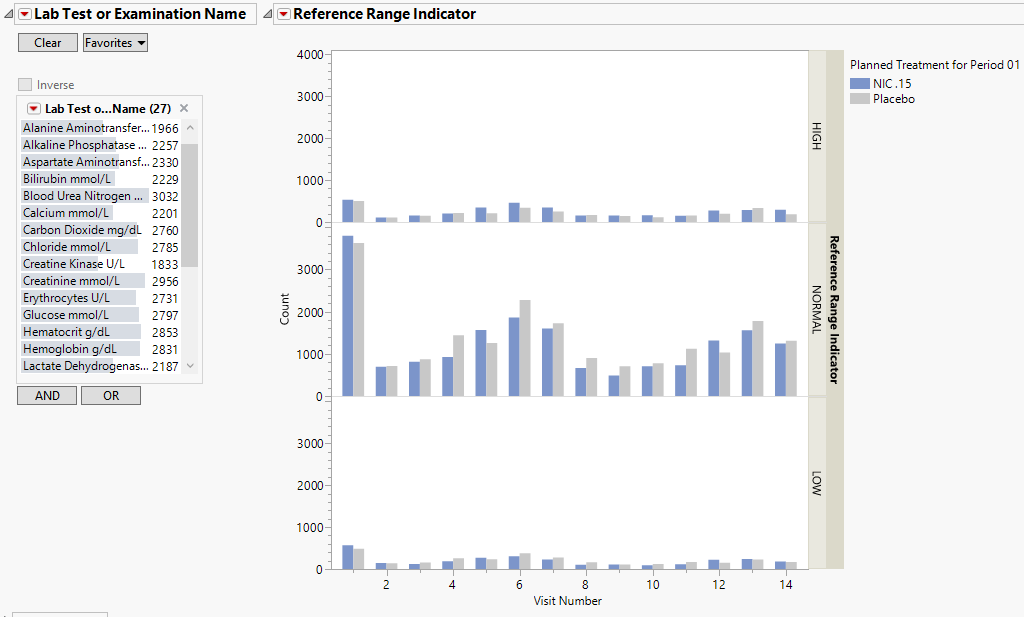
It contains the following elements:
| • | A set of count plots for each Findings Test that has nonmissing values for the xxNRIND variable. Select the test to be displayed using the data filter at left. |
These plots show the distribution of measurements across categories of the Reference Range Indicator variable (xxNRIND). For example, you can see how many laboratory measurements for a given test were categorized as HIGH, NORMAL, or LOW based on values of the Reference Range Upper Limit and Reference Range Lower Limit (LBSTNRLO and LBSTNRHI, respectively). The graph contains bars representing the counts within each category for each treatment across Study Visits (VISIT or VISITNUM).
Test Results
Contains One-way Analyses ( ANOVA) for each test that has numeric measurement results (xxSTRESN values), Contingency Analyses for each Findings test that has character results (xxSTRESC values but missing xxSTRESN values), or both.
Note: This section can display analyses for numeric and/or categorical findings tests, depending on the tests found within the chosen analysis Findings domain.
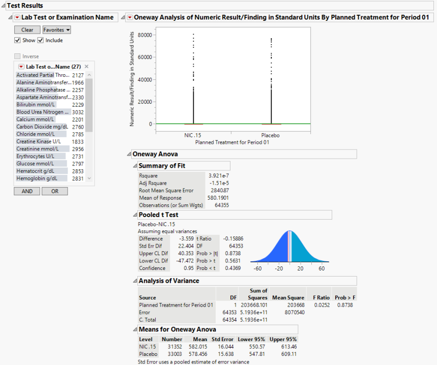
It contains one or both of the following elements:
| • | A set of Oneway Analyses for Numeric Findings Tests. |
Each analysis represents an Analysis of Variance (ANOVA) for each numeric Findings test (tests that contain nonmissing values for xxSTRESN) to compare measurements taken across different treatment arms. You can click the Oneway ANOVA outline box below each plot to show the statistical results of the analysis.
Note that, initially, this analysis is across all measurements taken during the study and should be used to get an idea of possibly significant differences in measurements across treatment arms. You can select individual tests to be displayed using the data filter at left. This is a simple model. You can fit a more appropriate model that accounts for the repeated measures taken for subjects, as well as initial baseline measurements, with the Findings ANOVA report.
See the JMP Fit Y by X platform for more details about Oneway Analysis.
Options
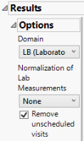
Domain
Use this widget to specify whether to plot the distribution of measurements from either the Electrocardiogram (EG), Laboratory (LB), or Vital Signs (VS) findings domains.
Normalization of Lab Measurements
Use this widget to select a normalization to be applied to the baseline and on-therapy measurements. Refer to Normalization of Lab Measurements for more information.
Remove unscheduled visits
You might or might not want to include unscheduled visits when you are analyzing findings by visit. Check the Remove unscheduled visits to exclude unscheduled visits.
General and Drill Down Buttons
Action buttons, provide you with an easy way to drill down into your data. The following action buttons are generated by this report:
| • | Click  to rerun the report using default settings. to rerun the report using default settings. |
| • | Click  to view the associated data tables. Refer to Show Tables/View Data for more information. to view the associated data tables. Refer to Show Tables/View Data for more information. |
| • | Click  to generate a standardized pdf- or rtf-formatted report containing the plots and charts of selected sections. to generate a standardized pdf- or rtf-formatted report containing the plots and charts of selected sections. |
| • | Click  to generate a JMP Live report. Refer to Create Live Report for more information. to generate a JMP Live report. Refer to Create Live Report for more information. |
| • | Click  to take notes, and store them in a central location. Refer to Add Notes for more information. to take notes, and store them in a central location. Refer to Add Notes for more information. |
| • | Click  to read user-generated notes. Refer to View Notes for more information. to read user-generated notes. Refer to View Notes for more information. |
| • | Click  to open and view the Subject Explorer/Review Subject Filter. to open and view the Subject Explorer/Review Subject Filter. |
| • | Click  to specify Derived Population Flags that enable you to divided the subject population into two distinct groups based on whether they meet very specific criteria. to specify Derived Population Flags that enable you to divided the subject population into two distinct groups based on whether they meet very specific criteria. |
Default Settings
Refer to Set Study Preferences for default Subject Level settings.
Methodology
No testing is performed. Analysis is restricted to tabulating counts/frequencies of subjects exhibiting constant findings results.