Dynamic Survival
The Dynamic Survival report provides a more informative and interactive experience for summarizing time-to-event endpoints from the ADTTE domain. The report uses JMP's Survival and Fit Proportional Hazards platforms to produce a Kaplan-Meier plot (either a survival or failure plot), annotations for the number of events (as well as the proportion of total events for Relative analyses), and a table for the number of patients at risk according to a user-supplied interval. A further enhancement of the Kaplan-Meier plot is that various statistics can be summarized using a second y-axis, including the log-rank and Wilcoxon tests, or hazard ratios between treatment arms from a corresponding proportional hazards model.
Report Results Description
Running Dynamic Survival for Nicardipine using default settings generates the report shown below. Output from the report is organized into sections. Each section contains one or more plots, data panels, data filters, or other elements that facilitate your analysis.
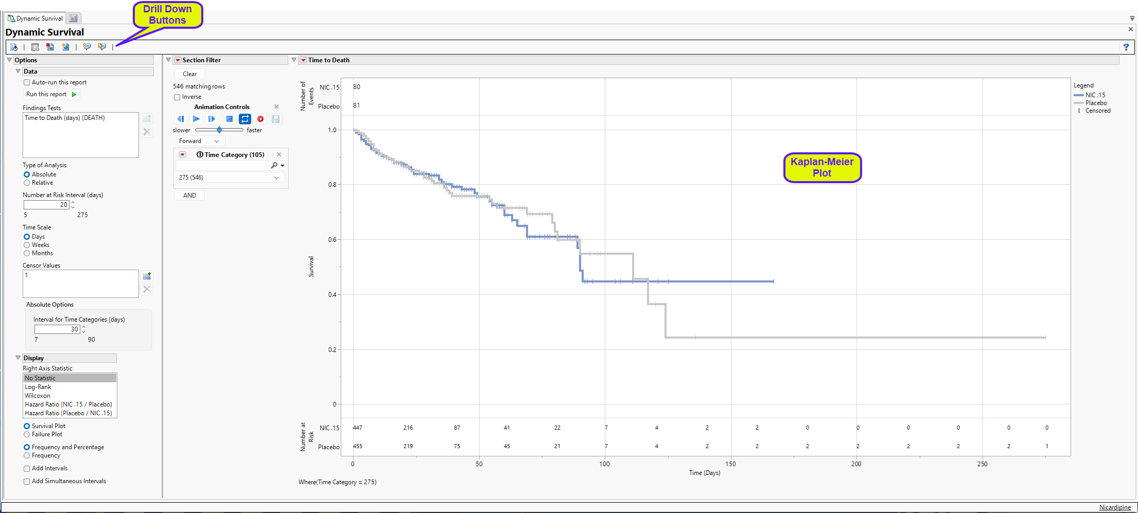
The report displays a survival plot summarizing a Relative analysis of the Nicardipine Time to Death endpoint from ADTTE. Censored observations are represented by the vertical pipe symbols. At the top of the figure, the total Number of Events experienced for each arm are summarized; the bottom of the figure presents a table for the Number of Patients at Risk in 20-day increments.
Number at Risk
This section of the plot indicates the number of subjects in each treatment arm still participating in the study at each interval specified using the Number at Risk Interval (days) option.
Sectional Filter
This data filter enables you to subset subjects based on time and other factors. You can select Time Category in the filter and use the animation controls to play an animation of how the survival analysis will change over time. Refer to Data Filter for more information.
Analyses
This report uses the JMP Survival and Fit Proportional Hazards platforms to analyze a single endpoint from the ADTTE domain. Essentially, the Survival and Fit Proportional Hazards platforms analyze survival endpoints separately for distinct time categories that are produced according to the type of analysis that is requested, Absolute or Relative (default).
Absolute Time
In this analysis, we observe survival data plotted by patient and date (see below). Each patient’s time (ADTTE.AVAL) is measured from a start date (ADTTE.STARTDT) to an end date (ADTTE.ADT) where the patient experiences an event (CNSR = 0) or is censored (CNSR > 0) for not having experienced an event prior to the end of follow-up.
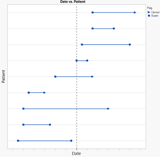
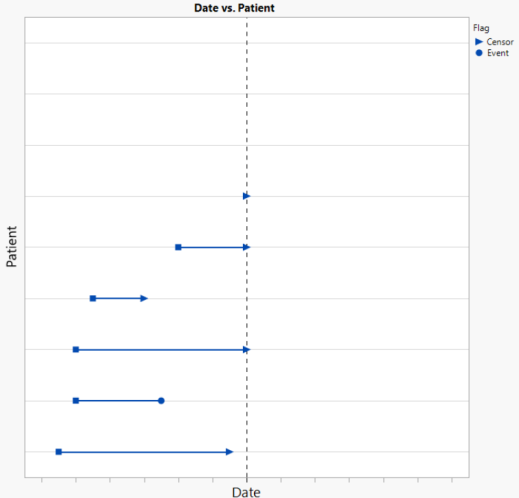
Suppose there was interest in conducting an interim analysis at a date indicated by the dashed horizontal reference line. For this analysis, patients whose follow-up extends beyond this reference date would be censored at this date (see below). This interim analysis conducted using this data would include 6 patients, only one of whom had an event prior to the reference date.
While it is typical to preplan for a small number of interim analyses to assess the outcome for a survival endpoint, there may be interest in understanding how robust the results are to the timing of the interim analysis. What if the analysis had been conducted 2-weeks earlier? 4- weeks? How would the results change? An Absolute analysis from this report enables you to answer this question easily. Based on the value specified using the Interval for Time Categories (days) option, the analyst can recompute the survival analysis in 7-90 day intervals counting backwards from the observed maximum event/censor date (ADTTE.ADT). Time Category values include dates according to this interval as long as the date is greater than the minimum event/censor date. Because the analysis is based on absolute time, patients may be excluded from Time Categories.
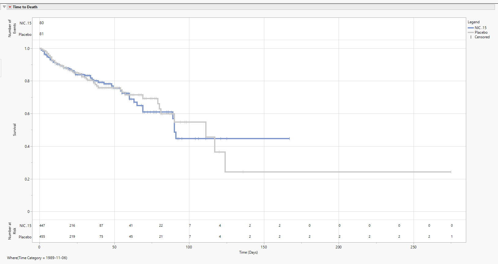
The figure below is an Absolute analysis of the Nicardipine Time to Death endpoint from ADTTE. Censored observations are represented by the vertical pipe symbols. At the top of the figure,
the total Number of Events experienced for each arm are summarized; the bottom of the figure presents a table for the Number of Patients at Risk in 20-day increments.
Additional Notes about the Absolute analyses
| • | Analyzing survival data on an absolute scale can be used to assess sensitivity of a survival analysis to the timing of an interim analysis. |
| • | In addition to changing the follow-up time to an event/censor outcome, the sample size can change as patients are excluded from analysis if the Time Category date precedes the start date. |
| • | Time Categories of a fixed number of days apart are produced counting backwards from the maximum event/censor date and stops prior to the minimum event/censor date. |
| • | Since knowledge of the start and event/censor dates is required to produce this analysis, time can be computed according to different units (Time Scale: days, weeks, months) and presented as such in the figure. |
| • | Statistics are summarized according to the maximum time observed according to the dates included in the Time Categories. It is natural to see statistics summarized at fewer times than there are dates in Time Categories. |
Relative Time
In contrast to the Absolute analysis described in Figure 2, the Relative analysis (see below) considers time within each patient relative to their start dates. Therefore, all patients start at time 0 (coinciding with ADTTE.STARTDT) and the number of days (most generally) to reach the event/censor date will coincide with ADTTE.ADT. In a manner similar to the Absolute analysis, suppose there was interest in conducting an analysis at a Relative time indicated by the dashed horizontal reference line.
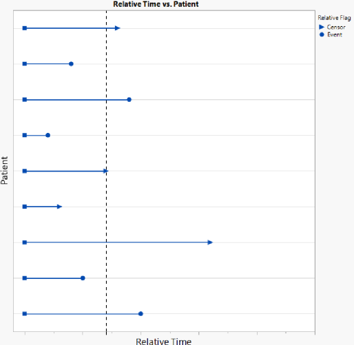
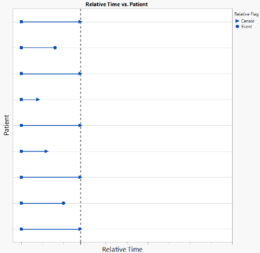
For this analysis, patients whose follow-up extends beyond this reference time would be censored at this time (see below). Unlike the absolute analysis, this analysis would include every patient, since every patient is included in the analysis since time 0.
The figure below shows a Relative analysis for Nicardipine for Time Category 100 (which can be thought of as 100 days of follow-up from Time 0). Both confidence intervals have been added to the figure as well as a line for the hazard ratio for Nicardipine vs. Placebo. By day 100, there are 7 patients still at risk for each treatment arm, and the initial sample sizes coincide with the total sample sizes of treated patients in each arm. Notice that the Number of Events includes the proportion of Total Events experienced for each arm. By day 100, all 80 events have been experienced on the NIC.15 arm, and 78 of 81 events (96.3%) have been experience on Placebo, indicating that there are 3 events left to occur by the end of the analysis.
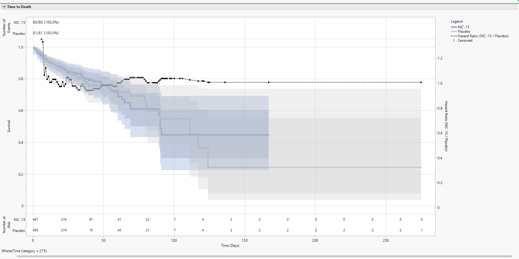
A Relative analysis makes it possible to view an animation and watch as the proportion of events grows over time. Note the Display tab has an additional button available called Frequency/Frequency and Percentage. This is to remove the percentages if it is of interest to save the plots for publication [saving 80/80 (100.0%) and 81/81 (100%) at the maximum Time Category isn’t particularly meaningful].
Additional Notes about the Relative analyses
| • | Analyzing survival data on a Relative scale can be used to assess sensitivity of statistics to accumulating data (such as statistical tests and proportional hazards). For example, plots can be used to assess whether Kaplan-Meier plots have constant proportional hazards across time. |
| • | Allows for proper animation of the changing survival/failure curves and for viewing of the proportion of total events over time. |
| • | Sample size does not change across the Time Categories since all patients are naturally included beginning at Time 0. |
| • | Unlike the Absolute analysis that computes Time Categories in user-supplied intervals from the maximum event censor date, a Relative analysis is recomputed at every observed event/censor time as Time Categories. |
| • | Knowledge of the start and event/censor dates are not required. Therefore, time is only presented according to the given units of the original data (which the user confirms in the dialog using Time Scale (Days is the default). |
| • | Because the Relative analysis is based on the time since start date (usually in days), the statistics are computed at each and every observed event/censor time. |
Options
Data
Auto-run this report
Check this box to auto-run the report upon launch. Previously saved settings are used.
Run this report
Use this widget to run this report after modifying any of the options. This option is not available when the Auto-run check box is checked.
Findings Tests
Use this widget to select specific Findings tests.
| 8 | Click  to open the Add window (shown below) that lists available test names (shown below). to open the Add window (shown below) that lists available test names (shown below). |
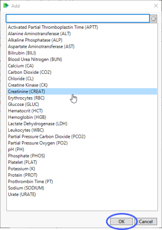
| 8 | Select the desired test(s) and click to add them to the text box. |
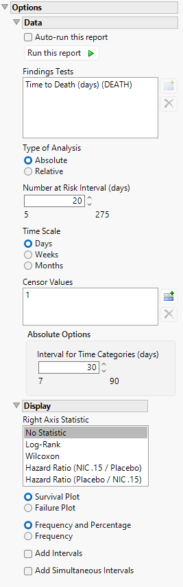
Type of Analysis
This option enables you to specify whether to show survival numbers in absolute ( based on the actual date) or relative (based on the number days a participant has participated in the study) terms.
Number at Risk Interval (days)
Enter the number of days comprising the block of time between study days where the number of subjects remaining in the study are reported.
Time Scale
Use this widget to specify the time scale to use for times. Options can include Hours, Days, Weeks, Months, and Years. Refer to Time Scale for more information.
Censor Values
Use this option to specify the flag value indicating whether a subject is censored and has left the study.
Interval for Time Categories (days)
This option enables you to specify a value that is used to create time blocks for assessing survival.
This option is available only when Absolute is specified as the type of analysis.
Display
Right Axis Statistic
Use this option to overlay a selected statistical plot on the survival plot. You can plot either of the p-values (from the Survival platform) or hazard ratios (from the Fit Proportional Hazards platform) across time by adding a second y-axis.
Survival/Failure Plot
This options enables you to toggle the display between showing a survival plot and failure plot.
Check Survival Plot to view a Kaplan-Meier plot. This curve is based on the survival function estimator calculated using clinical outcome data. It is used to measure the proportion of patients living for a given amount of time after treatment.
Check Failure Plot to display a failure plot, which contains overlaid failure curves (proportion failing over time) for each group. A failure plot, where the y-axis starts at 0 and increases upwards as events occur, reverses the vertical axis to show the number of failures rather than the number of survivors.
Frequency/Frequency and Percentage
Use this option to specify whether to include percentage of surviving subjects in each treatment arm along the frequency. This option is enabled only when a relative analysis is run.
Add Intervals
Check this option to show the 95% pointwise confidence bands for the Kaplan-Meier survival functions in the Survival Plot and the Failure Plot. Meeker and Escobar (1998, ch. 3) discuss pointwise and simultaneous confidence intervals and the motivation for simultaneous confidence intervals in survival analysis.
Add Simultaneous Intervals
Check this option to show the 95% simultaneous confidence bands for the Kaplan-Meier survival functions in the Survival Plot and the Failure Plot. Meeker and Escobar (1998, ch. 3) discuss pointwise and simultaneous confidence intervals and the motivation for simultaneous confidence intervals in survival analysis.
General and Drill Down Buttons
Action buttons provide you with an easy way to drill down into your data. The following action buttons are generated by this report:
| • | Click  to reset all report options to default settings. to reset all report options to default settings. |
| • | Click  to view the associated data tables. Refer to Show Tables for more information. to view the associated data tables. Refer to Show Tables for more information. |
| • | Click  to generate a standardized pdf- or rtf-formatted report containing the plots and charts of selected sections. to generate a standardized pdf- or rtf-formatted report containing the plots and charts of selected sections. |
| • | Click  to generate a JMP Live report. Refer to Create Live Report for more information. to generate a JMP Live report. Refer to Create Live Report for more information. |
| • | Click  to take notes, and store them in a central location. Refer to Add Notes for more information. to take notes, and store them in a central location. Refer to Add Notes for more information. |
| • | Click  to read user-generated notes. Refer to View Notes for more information. to read user-generated notes. Refer to View Notes for more information. |
Default Settings
Refer to Set Study Preferences for default Subject Level settings.
Methodology
Refer to the documentation for JMP's Survival and Fit Proportional Hazards platforms for information on the statistical methods used to assess survival.
References
Meeker, W. Q., and Escobar, L. A. (1998). Statistical Methods for Reliability Data. New York: John Wiley & Sons.